We have recently written several blogs covering how different cloud providers handle database failover. We compared failover performance in Amazon Aurora, Amazon RDS and ClusterControl, tested the failover behavior in Amazon RDS, and also on Google Cloud Platform. While those services provide great options when it comes to failover, they may not be right for every application.

In this blog post we will spend a bit of time analysing the pros and cons of using the DBaaS solutions compared with designing an environment manually or by using a database management platform, like ClusterControl.

Implementing High Availability Databases with Managed Solutions

The primary reason to use existing solutions is ease of use. You can deploy a highly available solution with automated failover in just a couple of clicks. There’s no need for combining different tools together, managing the databases by hand, deploying tools, writing scripts, designing the monitoring, or any other database management operations. Everything is already in place. This can seriously reduce the learning curve and requires less experience to set up a highly-available environment for the databases; allowing basically everyone to deploy such setups.

In most of the cases with these solutions, the failover process is executed within a reasonable time. It may be blazing fast as with Amazon Aurora or somewhat slower as with Google Cloud Platform SQL nodes. For the majority of the cases, these types of results are acceptable. 

The bottom line. If you can accept 30 - 60 seconds of downtime, you should be ok using any of the DBaaS platforms.

The Downside of Using a Managed Solution for HA

While DBaaS solutions are simple to use, they also come with some serious drawbacks. For starters, there is always a vendor lock-in component to consider. Once you deploy a cluster in Amazon Web Services it is quite tricky to migrate out of that provider. There are no easy methods to download the full dataset through a physical backup. With most providers, only manually executed logical backups are available. Sure, there are always options to achieve this, but it is typically a complex, time-consuming process, which still may require some downtime after all.

Using a provider like Amazon RDS also comes with limitations. Some actions cannot be easily performed which would be very simple to accomplish on environments deployed in a fully user-controlled manner (e.g. AWS EC2). Some of these limitations have already been covered in other blogs, but to summarize is that no DBaaS service gives you the same level of flexibility as regular MySQL GTID-based replication. You can promote any slave, you can re-slave every node off any other...virtually every action is possible. With tools like RDS you face design-induced limitations you cannot bypass.

The problem is also with an ability to understand performance details. When you design your own highly available setup, you become knowledgeable about potential performance issues that may show up. On the other hand, RDS and similar environments are pretty much “black boxes.” Yes, we have learned that Amazon RDS uses DRBD to create a shadow copy of the master, we know that Aurora uses shared, replicated storage to implement very fast failovers. That’s just a general knowledge. We cannot tell what are the performance implications of those solutions other than what we might casually notice. What are common issues associated with them? How stable are those solutions? Only the developers behind the solution know for sure.

What is the Alternative to DBaaS Solutions?

You may wonder, is there an alternative to DBaaS? After all, it is so convenient to run the managed service where you can access most of the typical actions via UI. You can create and restore backups, failover is handled automatically for you. The environment is easy-to-use which can be compelling for companies who do not have dedicated and experienced staff for dealing with databases.

ClusterControl provides a great alternative to cloud-based DBaaS services. It provides you with a graphical user interface, which can be used to deploy, manage, and monitor open source databases. 

In couple of clicks you can easily deploy a highly-available database cluster, with automated failover (faster than most of the DBaaS offerings), backup management, advanced monitoring, and other features like integration with external tools (e.g. Slack or PagerDuty) or upgrade management. All this while completely avoiding vendor lock-in. 

ClusterControl doesn’t care where your databases are located as long as it can connect to them using SSH. You can have setups in cloud, on-prem, or in a mixed environment of multiple cloud providers. As long as connectivity is there, ClusterControl will be able to manage the environment. Utilizing the solutions you want (and not the ones that you are not familiar nor aware of) allows you to take full control over the environment at any point in time. 

Whatever setup you deployed with ClusterControl, you can easily manage it in a more traditional, manual or scripted way. ClusterControl even provides you with command line interface, which will let you incorporate tasks executed by ClusterControl into your shell scripts. You have all the control you want - nothing is a black box, every piece of the environment would be built using open source solutions combined together and deployed by ClusterControl.

Let’s take a look at how easily you can deploy a MySQL Replication cluster using ClusterControl. Let’s assume you have the environment prepared with ClusterControl installed on one instance and all other nodes accessible via SSH from ClusterControl host.

We will start with picking the “Deploy” wizard.

At the first step we have to define how ClusterControl should connect to the nodes on which databases are to be deployed. Both root access or sudo (with or without the password) are supported.

Then, we want to pick a vendor, version and pass the password for the administrative user in our MySQL database.

Finally, we want to define the topology for our new cluster. As you can see, this is already quite complex setup, unlike something you can deploy using AWS RDS or GCP SQL node.

All we have to do now is to wait for the process to complete. ClusterControl will do its best to understand the environment it is deploying to and install required set of packages, including the database itself.

Once the cluster is up-and-running, you can proceed with deploying the proxy layer (which will provide your application with a single point of entry into the database layer). This is more or less what happens behind the scenes with DBaaS, where you also have endpoints to connect to the database cluster. It is quite common to use a single endpoint for writes and multiple endpoints for reaching particular replicas.

Here we will use ProxySQL, which will do the dirty work for us - it will understand the topology, sends writes only to the master and load balance read-only queries across all replicas that we have.

To deploy ProxySQL we will go to Manage -> Load Balancers.

We have to fill all required fields: hosts to deploy on, credentials for the administrative and monitoring user, we may import existing user from MySQL into ProxySQL or create a new one. All the details about ProxySQL can be easily found in multiple blogs in our blog section.

We want at least two ProxySQL nodes to be deployed to ensure high-availability. Then, once they are deployed, we will deploy Keepalived on top of ProxySQL. This will ensure that Virtual IP will be configured and pointing to one of the ProxySQL instances, as long as there will be at least one healthy node.

Here is the only potential problem if you go with cloud environments where routing works in a way that you cannot easily bring up a network interface. In such case you will have to modify the configuration of Keepalived, introduce ‘notify_master’ script and use a script, which will make the necessary IP changes - in case of EC2 it would have to detach Elastic IP from one host and attach it to the other host. 

There are plenty of instructions on how to do that using widely-tested open source software in setups deployed by ClusterControl. You can easily find additional information, tips, and how-to’s which are relevant to your particular environment.

Conclusion

We hope you found this blog post insightful. If you would like to test ClusterControl, it comes with a 30 day enterprise trial where you have available all the features. You can download it for free and test if it fits in your environment.

As soon as you start running a database server and your usage grows, you are exposed to many types of technical problems, performance degradation, and database malfunctions.  Each of these could lead to much bigger problems, such as catastrophic failure or data loss. It’s like a chain reaction, where one thing can lead to another, causing more and more issues. Proactive countermeasures must be performed in order for you to have a stable environment as long as possible.

In this blog post, we are going to look at a bunch of cool features offered by ClusterControl that can greatly help us troubleshoot and fix our MySQL database issues when they happen.

Database Alarms and Notifications

For all undesired events, ClusterControl will log everything under Alarms, accessible on the Activity (Top Menu) of ClusterControl page. This is commonly the first step to start troubleshooting when something goes wrong. From this page, we can get an idea on what is actually going on with our database cluster:

The above screenshot shows an example of a server unreachable event, with severity CRITICAL, detected by two components, Network and Node. If you have configured the email notifications setting, you should get a copy of these alarms in your mailbox. 

When clicking on the “Full Alarm Details,” you can get the important details of the alarm like hostname, timestamp, cluster name and so on. It also provides the next recommended step to take. You can also send out this alarm as an email to other recipients configured under the Email Notification Settings. 

You may also opt to silence an alarm by clicking the “Ignore Alarm” button and it will not appear in the list again. Ignoring an alarm might be useful if you have a low severity alarm and know how to handle or work around it. For example if ClusterControl detects a duplicate index in your database, where in some cases would be needed by your legacy applications.

By looking at this page, we can obtain an immediate understanding of what is going on with our database cluster and what the next step is to do to solve the problem. As in this case, one of the database nodes went down and became unreachable via SSH from the ClusterControl host. Even a beginner SysAdmin would now know what to do next if this alarm appears.

Centralized Database Log Files

This is where we can drill down what was wrong with our database server. Under ClusterControl -> Logs -> System Logs, you can see all log files related to the database cluster. As for MySQL-based database cluster, ClusterControl pulls the ProxySQL log, MySQL error log and backup logs:

Click on "Refresh Log" to retrieve the latest log from all hosts that are accessible at that particular time. If a node is unreachable, ClusterControl will still view the outdated log in since this information is stored inside the CMON database. By default ClusterControl keeps retrieving the system logs every 10 minutes, configurable under Settings -> Log Interval. 

ClusterControl will trigger the job to pull the latest log from each server, as shown in the following "Collect Logs" job:

A centralized view of log file allows us to have faster understanding on what went wrong. For a database cluster which commonly involves multiple nodes and tiers, this feature will greatly improve the log reading where a SysAdmin can compare these logs side-by-side and pinpoint critical events, reducing the total troubleshooting time. 

Web SSH Console

ClusterControl provides a web-based SSH console so you can access the DB server directly via the ClusterControl UI (as the SSH user is configured to connect to the database hosts). From here, we can gather much more information which allows us to fix the problem even faster. Everyone knows when a database issue hits the production system, every second of downtime counts.

To access the SSH console via web, simply pick the nodes under Nodes -> Node Actions -> SSH Console, or simply click on the gear icon for a shortcut:

Due to security concern that might be imposed with this feature, especially for multi-user or multi-tenant environment, one can disable it by going to /var/www/html/clustercontrol/bootstrap.php on ClusterControl server and set the following constant to false:

define('SSH_ENABLED', false);

Refresh the ClusterControl UI page to load the new changes.

Database Performance Issues

Apart from monitoring and trending features, ClusterControl proactively sends you various alarms and advisors related to database performance, for example:

• Excessive usage - Resource that passes certain thresholds like CPU, memory, swap usage and disk space.
• Cluster degradation - Cluster and network partitioning.
• System time drift - Time difference among all nodes in the cluster (including ClusterControl node).
• Various other MySQL related advisors:
  • Replication - replication lag, binlog expiration, location and growth
  • Galera - SST method, scan GRA logfile, cluster address checker
  • Schema check - Non-transactional table existance on Galera Cluster.
  • Connections - Threads connected ratio
  • InnoDB - Dirty pages ratio, InnoDB log file growth
  • Slow queries - By default ClusterControl will raise an alarm if it finds a query running for more than 30 seconds. This is of course configurable under Settings -> Runtime Configuration -> Long Query.
  • Deadlocks - InnoDB transactions deadlock and Galera deadlock.
  • Indexes - Duplicate keys, table without primary keys.

Check out the Advisors page under Performance -> Advisors to get the details of things that can be improved as suggested by ClusterControl. For every advisor, it provides justifications and advice as shown in the following example for "Checking Disk Space Usage" advisor:

When a performance issue occurs you will get "Warning" (yellow) or "Critical" (red) status on these advisors. Further tuning is commonly required to overcome the problem. Advisors raise alarms, which means, users will get a copy of these alarms inside the mailbox if Email Notifications are configured accordingly. For every alarm raised by ClusterControl or its advisors, users will also get an email if the alarm has been cleared. These are pre-configured within ClusterControl and require no initial configuration. Further customization is always possible under Manage -> Developer Studio. You can check out this blog post on how to write your own advisor.

ClusterControl also provides a dedicated page in regards to database performance under ClusterControl -> Performance. It provides all sorts of database insights following the best-practices like centralized view of DB Status, Variables, InnoDB status, Schema Analyzer, Transaction Logs. These are pretty self-explanatory and straightforward to understand.

For query performance, you can inspect Top Queries and Query Outliers, where ClusterControl highlights queries which performed significantly differ from their average query. We have covered this topic in detail in this blog post, MySQL Query Performance Tuning.

Database Error Reports

ClusterControl comes with an error report generator tool, to collect debugging information about your database cluster to help understand the current situation and status. To generate an error report, simply go to ClusterControl -> Logs -> Error Reports -> Create Error Report:

The generated error report can be downloaded from this page once ready. This generated report will be in TAR ball format (tar.gz) and you may attach it to a support request. Since the support ticket has the limit of 10MB of file size, if the tarball size is bigger than that, you could upload it into a cloud drive and only share with us the download link with proper permission. You may remove it later once we already got the file. You can also generate the error report via command line as explained in the Error Report documentation page.

In the event of an outage, we highly recommend that you generate multiple error reports during and right after the outage. Those reports will be very useful to try to understand what went wrong, the consequences of the outage, and to verify that the cluster is in-fact back to operational status after a disastrous event.

Conclusion

ClusterControl proactive monitoring, together with a set of troubleshooting features, provide an efficient platform for  users to troubleshoot any kind of MySQL database issues. Long gone is the legacy way of troubleshooting where one has to open multiple SSH sessions to access multiple hosts and execute multiple commands repeatedly in order to pinpoint the root cause.

If the above mentioned features are not helping you in solving the problem or troubleshooting the database issue, you always contact the Severalnines Support Team to back you up. Our 24/7/365 dedicated technical experts are available to attend your request at anytime. Our average first reply time is usually less than 30 minutes.

MySQL Galera Cluster 4.0 is the new kid on the database block with very interesting new features. Currently it is available only as a part of MariaDB 10.4 but in the future it will work as well with MySQL 5.6, 5.7 and 8.0. In this blog post we would like to go over some of the new features that came along with Galera Cluster 4.0.

Galera Cluster Streaming Replication

The most important new feature in this release is streaming replication. So far the certification process for the Galera Cluster worked in a way that whole transactions had to be certified after they completed. 

This process was not ideal in several scenarios...

1. Hotspots in tables, rows which are very frequently updated on multiple nodes - hundreds of fast transactions running on multiple nodes, modifying the same set of rows result in frequent deadlocks and rollback of transactions
2. Long running transactions - if a transaction takes significant time to complete, this seriously increases chances that some other transaction, in the meantime, on another node, may modify some of the rows that were also updated by the long transaction. This resulted in a deadlock during certification and one of the transactions having to be rolled back.
3. Large transactions - if a transaction modifies a significant number of rows, it is likely that another transaction, at the same time, on a different node, will modify one of the rows already modified by the large transaction. This results in a deadlock during certification and one of the transactions has to be rolled back. In addition to this, large transactions will take additional time to be processed, sent to all nodes in the cluster and certified. This is not an ideal situation as it adds delay to commits and slows down the whole cluster.

Luckily, streaming replication can solve these problems. The main difference is that the certification happens in chunks where there is no need to wait for the whole transaction to complete. As a result, even if a transaction is large or long, majority (or all, depending on the settings we will discuss in a moment) of rows are locked on all of the nodes, preventing other queries from modifying them.

MySQL Galera Cluster Streaming Replication Options

There are two configuration options for streaming replication: 

wsrep_trx_fragment_size 

This tells how big a fragment should be (by default it is set to 0, which means that the streaming replication is disabled)

wsrep_trx_fragment_unit 

This tells what the fragment really is. By default it is bytes, but it can also be a ‘statements’ or ‘rows’. 

Those variables can (and should) be set on a session level, making it possible for user to decide which particular query should be replicated using streaming replication. Setting unit to ‘statements’ and size to 1 allow, for example, to use streaming replication just for a single query which, for example, updates a hotspot.

You can configure Galera 4.0 to certify every row that you have modified and grab the locks on all of the nodes while doing so. This makes streaming replication great at solving problems with frequent deadlocks which, prior to Galera 4.0, were possible to solve only by redirecting all writes to a single node.

WSREP Tables

Galera 4.0 introduces several tables, which will help to monitor the state of the cluster:

• wsrep_cluster
• wsrep_cluster_members
• wsrep_streaming_log

All of them are located in the ‘mysql’ schema. wsrep_cluster will provide insight into the state of the cluster. wsrep_cluster_members will give you information about the nodes that are part of the cluster. wsrep_streaming_log helps to track the state of the streaming replication.

Galera Cluster Upcoming Features

Codership, the company behind the Galera, isn’t done yet. We were able to get a preview of the roadmap  from CEO, Seppo Jaakola which was given at Percona Live earlier this year. Apparently, we are going to see features like XA transaction support and gcache encryption. This is really good news. 

Support for XA transactions will be possible thanks to the streaming replication. In short, XA transactions are the distributed transactions which can run across multiple nodes. They utilize two-phase commit, which requires to first acquire all required locks to run the transaction on all of the nodes and then, once it is done, commit the changes. In previous versions Galera did not have means to lock resources on remote nodes, with streaming replication this has changed.

Gcache is a file which stores writesets. Its contents are sent to joiner nodes which asks for a data transfer. If all data is stored in the gcache, joiner will receive just the missing transactions in the process called Incremental State Transfer (IST). If gcache does not contain all required data, State Snapshot Transfer (SST) will be required and the whole dataset will have to be transferred to the joining node. 

Gcache contains information about recent changes, therefore it’s great to see its contents encrypted for better security. With better security standards being introduced through more and more regulations, it is crucial that the software will become better at achieving compliance.

Conclusion

We are definitely looking forward to see how Galera Cluster 4.0 will work out on databases than MariaDB. Being able to deploy MySQL 5.7 or 8.0 with Galera Cluster will be really great. After all, Galera is one of the most widely tested synchronous replication solutions that are available on the market.

PostgreSQL can work separately on multiple machines with the same data structure, making the persistence layer of the application more resilient and prepared for some unexpected event that might compromise the continuity of the service.

The idea behind this is to improve the system response time by distributing the requests in a “Round Robin” network where each node present is a cluster. In this type of setup it is not important as to which one the requests will be delivered to be processed, as the response would always be the same.

In this blog, we will explain how to replicate a PostgreSQL cluster using the tools provided in the program installation. The version used is PostgreSQL 11.5, the current stable,  generally-available version for the operating system Debian Buster. For the examples in this blog it is assumed that you are already familiar with Linux.

PostgreSQL Programs

Inside the directory /usr/bin/ is the program responsible for managing the cluster.

# 1. Lists the files contained in the directory
# 2. Filters the elements that contain 'pg_' in the name
ls /usr/bin/ | grep pg_

Activities conducted through these programs can be performed sequentially, or even in combination with other programs. Running a block of these activities through a single command is possible thanks to a Linux program found in the same directory, called make.

To list the clusters present use the pg_lsclusters program. You can also use make to run it. Its work depends on a file named Makefile, which needs to be in the same directory where the command will run.

# 1. The current directory is checked
pwd

# 2. Creates a directory
mkdir ~/Documents/Severalnines/

# 3. Enroute to the chosen directory
cd ~/Documents/Severalnines/

# 4. Create the file Makefile
touch Makefile

# 5. Open the file for editing

The definition of a block is shown below, having as its name ls, and a single program to be run, pg_lsclusters.

# 1. Block name
ls:
# 2. Program to be executed
pg_lsclusters

The file Makefile can contain multiple blocks, and each can run as many programs as you need, and even receive parameters. It is imperative that the lines belonging to a block of execution are correct, using tabulations for indenting instead of spaces.

The use of make to run the pg_lsclusters program is accomplished by using the make ls command.

# 1. Executes pg_lsclusters
make ls

The result obtained in a recent PostgreSQL installation brings a single cluster called main, allocated on port 5432 of the operating system. When the pg_createcluster program is used, a new port is allocated to the new cluster created, having the value 5432 as the starting point, until another is found in ascending order.

Write Ahead Logging (WAL)

This replication procedure consists of making a backup of a working cluster which is continuing to receive updates. If this is done on the same machine, however, many of the benefits brought by this technique are lost.

Scaling a system horizontally ensures greater availability of the service, as if any hardware problems occur, it wouldn’t make much difference as there are other machines ready to take on the workload.

WAL is the term used to represent an internal complex algorithm to PostgreSQL that ensures the integrity of the transactions that are made on the system. However, only a single cluster must have the responsibility to access it with write permission.

The architecture now has three distinct types of clusters:

1. A primary with responsibility for writing to WAL;
2. A replica ready to take over the primary post;
3. Miscellaneous other replicas with WAL reading duty.

Write operations are any activities that are intended to modify the data structure, either by entering new elements, or updating and deleting existing records.

PostgreSQL Cluster Configuration

Each cluster has two directories, one containing its configuration files and another with the transaction logs. These are located in /etc/postgresql/11/$(cluster) and /var/lib/postgresql/11/$(cluster), respectively (where $(cluster) is the name of the cluster).

The file postgresql.conf is created immediately after the cluster has been created by running the program pg_createcluster, and the properties can be modified for the customization of a cluster.

Editing this file directly is not recommended because it contains almost all properties. Their values have been commented out, having the symbol # at the beginning of each line, and several other lines commented out containing instructions for changing the property values.

Adding another file containing the desired changes is possible, simply edit a single property named include, replacing the default value #include = ‘’ with include = ‘postgresql.replication.conf’.

Before you start the cluster, you need the presence of the file postgresql.replication.conf in the same directory where you find the original configuration file, called postgresql.conf.

# 1. Block name
create:
# 2. Creates the cluster
pg_createcluster 11 $(cluster) -- --data-checksums
# 3. Copies the file to the directory
cp postgresql.replication.conf /etc/postgresql/11/$(cluster)/
# 4. A value is assigned to the property
sed -i "s|^#include = ''|include = 'postgresql.replication.conf'|g" /etc/postgresql/11/$(cluster)/postgresql.conf

The use of --data-checksums in the creation of the cluster adds a greater level of integrity to the data, costing a bit of performance but being very important in order to avoid corruption of the files when transferred from one cluster to another.

The procedures described above can be reused for other clusters, simply passing a value to $(cluster) as a parameter in the execution of the program make.

# 1. Executes the block 'create' by passing a parameter
sudo make create cluster=primary

Now that a brief automation of the tasks has been established, what remains to be done is the definition of the file postgresql.replication.conf according to the need for each cluster.

Replication on PostgreSQL

Two ways to replicate a cluster are possible, one being complete the other involving the entire cluster (called Streaming Replication) and another could partial or complete (called Logical Replication).

The settings that must be specified for a cluster fall into four main categories:

• Master Server
• Standby Servers
• Sending Servers
• Subscribers

As we saw earlier, WAL is a file that contains the transactions that are made on the cluster, and the replication is the transmission of these files from one cluster to another.

Inside the settings present in the file postgresql.conf, we can see properties that define the behavior of the cluster in relation to the WAL files, such as the size of those files.

# default values
max_wal_size = 1GB
min_wal_size = 80MB

Another important property called max_wal_senders. Belonging to a cluster with characteristic Sending Servers, is the amount of processes responsible for sending these files to other clusters, having to always a value more than the number of clusters that depend on their receipt.

WAL files can be stored for transmission to a cluster that connects late, or that has had some problems in receiving it, and need previous files in relation to the current time, having the property wal_keep_segments as the specification for how many WAL file segments are to be maintained by a cluster.

A Replication Slot is a functionality that allows the cluster to store WAL files needed to provide another cluster with all the records, having the max_replication_slots option as its property.

# default values
max_wal_senders = 10
wal_keep_segments = 0
max_replication_slots = 10

When the intention is to outsource the storage of these WAL files, another method of processing these files can be used, called Continuous Archiving.

Continuous Archiving

This concept allows you to direct the WAL files to a specific location, using a Linux program, and two variables representing the path of the file, and its name, such as %p, and %f, respectively.

This property is disabled by default, but its use can be easily implemented by withdrawing the responsibility of a cluster from storing such important files, and can be added to the file postgresql.replication.conf.

# 1. Creates a directory
mkdir ~/Documents/Severalnines/Archiving

# 2. Implementation on postgresql.replication.conf
archive_mode = on
archive_command = 'cp %p ~/Documents/Severalnines/Archiving/%f'

# 3. Starts the cluster
sudo systemctl start postgresql@11-primary

After the cluster initialization, some properties might need to be modified, and a cluster restart could be required. However, some properties can only be reloaded, without the need for a full reboot of a cluster.

Information on such subjects can be obtained through the comments present in the file postgresql.conf, appearing as # (note: change requires restart).

If this is the case, a simple way to resolve is with the Linux program systemctl, used previously to start the cluster, having only to override the option to restart.

When a full reboot is not required, the cluster itself can reassign its properties through a query run within itself, however, if multiple clusters are running on the same machine, it will be required to pass a parameter containing the port value that the cluster is allocated on the operating system.

# Reload without restarting
sudo -H -u postgres psql -c ‘SELECT pg_reload_conf();’ -p 5433

In the example above, the property archive_mode requires a reboot, while archive_command does not. After this brief introduction to this subject, let’s look at how a replica cluster can backup these archived WAL files, using Point In Time Recovery (PITR).

PostgreSQL Replication Point-In-Time Recovery

This suggestive name allows a cluster to go back to its state from a certain period in time. This is done through a property called recovery_target_timeline, which expects to receive a value in date format, such as 2019-08-22 12:05 GMT, or the assignment latest, informing the need for a recovery up to the last existing record.

The program pg_basebackup when it runs, makes a copy of a directory containing the data from a cluster to another location. This program tends to receive multiple parameters, being one of them -R, which creates a file named recovery.conf within the copied directory, which in turn is not the same as that contains the other configuration files previously seen, such as postgresql.conf.

The file recovery.conf stores the parameters passed in the execution of the program pg_basebackup, and its existence is essential to the Streaming Replication implementation, because it is within it that the reverse operation to the Continuous Archiving can be performed.

# 1. Block name
replicate:
# 2. Removes the current data directory
rm -rf /var/lib/postgresql/11/$(replica)
# 3. Connects to primary cluster as user postgres
# 4. Copies the entire data directory
# 5. Creates the file recovery.conf
pg_basebackup -U postgres -d postgresql://localhost:$(primaryPort) -D /var/lib/postgresql/11/$(replica) -P -R
# 6. Inserts the restore_command property and its value
echo "restore_command = 'cp ~/Documents/Severalnines/Archiving/%f %p'">> /var/lib/postgresql/11/$(replica)/recovery.conf
# 7. The same is done with recovery_target_timeline
echo "recovery_target_timeline = 'latest'">> /var/lib/postgresql/11/$(replica)/recovery.conf

This replicate block specified above needs to be run by the operating system’s postgres user, in order to avoid potential conflicts with who is the owner of the cluster data, postgres, or the user root.

The replica cluster is still standing, basting it to successfully start the replication, having the replica cluster process called pg_walreceiver interacting with the primary cluster called pg_walsender over a TCP connection.

# 1. Executes the block ‘replicate’ by passing two parameters
sudo -H -u postgres make replicate replica=replica primaryPort=5433
# 2. Starts the cluster replica
sudo systemctl start postgresql@11-replica

Verification of the health of this replication model, called Streaming Replication, is performed by a query that is run on the primary cluster.

# 1. Checks the Streaming Replication created
sudo -H -u postgres psql -x -c ‘select * from pg_stat_replication;’ -p 5433

Conclusion

In this blog, we showed how to setup asynchronous Streaming Replication between two PostgreSQL clusters. Remember though, vulnerabilities exist in the code above, for example, using the postgres user to do such a task is not recommended.

The replication of a cluster provides several benefits when it is used in the correct way and has easy access to the APIs that come to interact with the clusters.

When it comes to backups and data archiving, IT departments are under pressure to meet stricter service level agreements, deliver more custom reports, and adhere to expanding compliance requirements while continuing to manage daily archive and backup tasks.  With no doubt, database server stores some of your enterprise’s most valuable information. Guaranteeing reliable database backups to prevent data loss in the event of an accident or hardware failure is a critical checkbox.

But how to make it truly DR when all of your data is in the single data center or even data centers that are in the near geolocation? Moreover, whether it is a 24x7 highly loaded server or a low-transaction-volume environment, you will be in the need of making backups a seamless procedure without disrupting the performance of the server in a production environment.

In this blog, we are going to review MongoDB backup to the cloud. The cloud has changed the data backup industry. Because of its affordable price point, smaller businesses have an offsite solution that backs up all of their data.

We will show you how to perform safe MongoDB backups using mongo services as well as other methods that you can use to extend your database disaster recovery options.

If your server or backup destination is located in an exposed infrastructure like a public cloud, hosting provider or connected through an untrusted WAN network, you need to think about additional actions in your backup policy. There are a few different ways to perform database backups for MongoDB, and depending on the type of backup, recovery time, size, and infrastructure options will vary. Since many of the cloud storage solutions are simply storage with different API front ends, any backup solution can be performed with a bit of scripting. So what are the options we have to make the process smooth and secure?

MongoDB Backup Encryption

Security should be in the center of every action IT teams do. It is always a good idea to enforce encryption to enhance the security of backup data. A simple use case to implement encryption is where you want to push the backup to offsite backup storage located in the public cloud.

When creating an encrypted backup, one thing to keep in mind is that it usually takes more time to recover. The backup has to be decrypted before any recovery activities. With a big dataset, this could introduce some delays to the RTO.

On the other hand, if you are using the private keys for encryption, make sure to store the key in a safe place. If the private key is missing, the backup will be useless and unrecoverable. If the key is stolen, all created backups that use the same key would be compromised as they are no longer secured. You can use popular GnuPG or OpenSSL to generate private or public keys.

To perform MongoDBdump encryption using GnuPG, generate a private key and follow the wizard accordingly:

$ gpg --gen-key

$ mongodump –db db1 –gzip –archive=/tmp/db1.tar.gz

$ gpg --encrypt -r ‘admin@email.com’ db1.tar.gz

$ rm -f db1.tar.gz

simply run the gpg command with --decrypt flag:

$ gpg --output db1.tar.gz --decrypt db1.tar.gz.gpg

OpenSSL req -x509 -nodes -newkey rsa:2048 -keyout dump.priv.pem -out dump.pub.pem

This private key (dump.priv.pem) must be kept in a safe place for future decryption. For Mongodump, an encrypted backup can be created by piping the content to openssl, for example

mongodump –db db1 –gzip –archive=/tmp/db1.tar.gz | openssl smime -encrypt -binary -text -aes256

-out database.sql.enc -outform DER dump.pub.pem

openssl smime -decrypt -in database.sql.enc -binary -inform

DEM -inkey dump.priv.pem -out db1.tar.gz

MongoDB Backup Compression

Within the database cloud backup world, compression is one of your best friends. It can not only save storage space, but it can also significantly reduce the time required to download/upload data.

In addition to archiving, we’ve also added support for compression using gzip. This is exposed by the introduction of a new command-line option “--gzip” in both mongodump and mongorestore. Compression works both for backups created using the directory and the archive mode and reduces disk space usage.

Normally, MongoDB dump can have the best compression rates as it is a flat text file. Depending on the compression tool and ratio, a compressed MongoDBdump can be up to 6 times smaller than the original backup size. To compress the backup, you can pipe the MongoDBdump output to a compression tool and redirect it to a destination file

Having a compressed backup could save you up to 50% of the original backup size, depending on the dataset. 

mongodump --db country --gzip --archive=country.archive

Limiting Network Throughput

A great option for cloud backups is to limit network streaming bandwidth (Mb/s) when doing a backup. You can achieve that with pv tool. The pv utility comes with data modifiers option -L RATE, --rate-limit RATE which limit the transfer to a maximum of RATE bytes per second. Below example will restrict it to 2MB/s.

$ pv -q -L 2m

Transferring MongoDB Backups to the Cloud

Now when your backup is compressed and secured (encrypted), it is ready for transfer.

Google Cloud

The gsutil command-line tool is used to manage, monitor and use your storage buckets on Google Cloud Storage. If you already installed the gcloud util, you already have the gsutil installed. Otherwise, follow the instructions for your Linux distribution from here.

To install the gcloud CLI you can follow the below procedure:

curl https://sdk.cloud.google.com | bash

exec -l $SHELL

gcloud init

gsutil mb -c regional -l europe-west1 gs://severalnines-storage/

Creating gs://MongoDB-backups-storage/

Amazon S3

If you are not using RDS to host your databases, it is very probable that you are doing your own backups. Amazon’s AWS platform, S3 (Amazon Simple Storage Service) is a data storage service that can be used to store database backups or other business-critical files. Either it’s Amazon EC2 instance or your on-prem environment you can use the service to secure your data.

While backups can be uploaded through the web interface, the dedicated s3 command line interface can be used to do it from the command line and through backup automation scripts. If backups are to be kept for a very long time, and recovery time isn’t a concern, backups can be transferred to Amazon Glacier service, providing much cheaper long-term storage. Files (amazon objects) are logically stored in a huge flat container named bucket. S3 presents a REST interface to its internals. You can use this API to perform CRUD operations on buckets and objects, as well as to change permissions and configurations on both.

The primary distribution method for the AWS CLI on Linux, Windows, and macOS is pip, a package manager for Python. Instructions can be found here.

aws s3 cp severalnines.sql s3://severalnine-sbucket/MongoDB_backups

Microsoft Azure Storage

Microsoft’s public cloud platform, Azure, has storage options with its control line interface. Information can be found here. The open-source, cross-platform Azure CLI provides a set of commands for working with the Azure platform. It gives much of the functionality seen in the Azure portal, including rich data access.

The installation of Azure CLI is fairly simple, you can find instructions here. Below you can find how to transfer your backup to Microsoft storage.

az storage blob upload --container-name severalnines --file severalnines.gz.tar --name severalnines_backup

Hybrid Storage for MongoDB Backups

With the growing public and private cloud storage industry, we have a new category called hybrid storage. The typical approach is to keep data on local disk drives for a shorter period while cloud backup storage would be held for a longer time. Many times the requirement for longer backup retention comes from legal obligations for different industries (like telecoms having to store connection metadata).This technology allows the files to be stored locally, with changes automatically synced to remote in the cloud. Such an approach is coming from the need of having recent backups stored locally for fast restore (lower RTO), as well as business continuity objectives.

The important aspect of efficient resource usage is to have separate backup retentions. Data that is stored locally, on redundant disk drives would be kept for a shorter period while cloud backup storage would be held for a longer time. Many times the requirement for longer backup retention comes from legal obligations for different industries (like telecoms having to store connection metadata).

Cloud providers like Google Cloud Services, Microsoft Azure and Amazon S3 each offer virtually unlimited storage, decreasing local space needs. It allows you to retain your backup files longer, for as long as you would like and not have concerns around local disk space.

ClusterControl Backup Management - Hybrid Storage

When scheduling backup with ClusterControl, each of the backup methods are configurable with a set of options on how you want the backup to be executed. The most important for the hybrid cloud storage would be:

• Network throttling
• Encryption with the built-in key management
• Compression
• The retention period for the local backups
• The retention period for the cloud backups

ClusterControl advanced backup features for cloud, parallel compression, network bandwidth limit, encryption, etc. Your company can take advantage of cloud scalability and pay-as-you-go pricing for growing storage needs. You can design a backup strategy to provide both local copies in the datacenter for immediate restoration, and a seamless gateway to cloud storage services from AWS, Google and Azure.

Advanced TLS and AES 256-bit encryption and compression features support secure backups that take up significantly less space in the cloud.

All companies nowadays have (or should have) a Disaster Recovery Plan (DRP) to prevent data loss in the case of failure; built according to an acceptable Recovery Point Objective (RPO) for the business.

A backup is a basic start in any DRP, but to guarantee the backup usability a single backup is just not enough. The best practice is to store the backup files in three different places, one stored locally on the database server (for faster recovery), another one in a centralized backup server, and the last one the cloud. For this last step, you should choose a stable and robust cloud provider to make sure your data is stored correctly and is accessible at any time.

In this blog, we will take a look at one of the most famous cloud providers, Google Cloud Platform (GCP) and how to use it to store your PostgreSQL backups in the cloud.

About Google Cloud

Google Cloud offers a wide range of products for your workload. Let’s look at some of them and how they are related to storing PostgreSQL backups in the cloud.

• Cloud Storage: It allows for world-wide storage and retrieval of any amount of data at any time. You can use Cloud Storage for a range of scenarios including serving website content, storing data for archival and disaster recovery, or distributing large data objects to users via direct download.
• Cloud SQL: It’s a fully managed database service that makes it easy to set up, maintain, manage, and administer your relational PostgreSQL, MySQL, and SQL Server databases in the cloud.
• Compute Engine: It delivers virtual machines running in Google Cloud with support to scaling from single instances to global, load-balanced cloud computing. Compute Engine's VMs boot quickly, come with high-performance persistent and local disk options, and deliver consistent performance. 

Storing Backups on Google Cloud

If you’re running your PostgreSQL database on Google Cloud with Cloud SQL you can back it up directly from the Google Cloud Platform, however, it’s not necessary to run it here to store your PostgreSQL backups.

Google Cloud Storage

Similar to the well-known Amazon S3 product, if you’re not running your PostgreSQL database with Cloud SQL, this is the most commonly used option to store backups or files in Google Cloud. It’s accessible from the Google Cloud Platform, in the Getting Started section or under the Storage left menu. With Cloud Storage, you can even easily transfer your S3 content here using the Transfer feature.

How to Use Google Cloud Storage

First, you need to create a new Bucket to store your data, so go toGoogle Cloud Platform -> Storage -> Create Bucket

In the first step, you need to just add a new bucket name.

In the next step, you can specify the location type (multi-region by default) and the location place.

Then, you can change the storage class from standard (default option) to nearline or coldline.

And then, you can change the control access.

Finally, you have some optional settings like encryption or retention policy.

Now you have your new bucket created, we will see how to use it.

Using the GSutil Tool

GSutil is a Python application that lets you access Cloud Storage from the command line. It allows you to perform different bucket and object management tasks. Let’s see how to install it on CentOS 7 and how to upload a backup using it.

Download Cloud SDK:

$ curl https://sdk.cloud.google.com | bash

Restart your shell:

$ exec -l $SHELL

Run gcloud init and configure the tool:

$ gcloud init

This command will ask you to login to your Google Cloud account by accessing a URL and adding an authentication code.

Now you have the tool installed and configured, let’s upload a backup to the bucket.

First, let’s check our buckets created:

[root@PG1bkp ~]# gsutil ls

gs://pgbackups1/

And to copy your PostgreSQL backup (or another file), run:

[root@PG1bkp ~]# gsutil cp /root/backups/BACKUP-3/base.tar.gz gs://pgbackups1/new_backup/

Copying file:///root/backups/BACKUP-3/base.tar.gz [Content-Type=application/x-tar]...

| [1 files][  4.9 MiB/ 4.9 MiB]

Operation completed over 1 objects/4.9 MiB.

The destination bucket must exist. 

And then, you can list the contents of the new_backup directory, to check the file uploaded:

[root@PG1bkp ~]# gsutil ls -r gs://pgbackups1/new_backup/*

gs://pgbackups1/new_backup/

gs://pgbackups1/new_backup/base.tar.gz

For more information about the GSutil usage, you can check the official documentation.

Google Cloud SQL

If you want to centralize all the environment (database + backups) into Google Cloud, you have available this Cloud SQL product. In this way, you will have your PostgreSQL database running on Google Cloud and you can also manage the backups from the same platform. It’s accessible from the Google Cloud Platform, in the Getting started section or under the Storage left menu.

How to Use Google Cloud SQL

To create a new PostgreSQL instance, go toGoogle Cloud Platform -> SQL -> Create Instance

Here you can choose between MySQL and PostgreSQL as the database engine. For this blog, let’s create a PostgreSQL instance.

Now, you need to add an instance ID, password, location and PostgreSQL version (9.6 or 11).

You have also some configuration options, like enable Public IP Address, Machine type and storage, and backups, etc. 

When the Cloud SQL instance is created, you can select it and you will see an overview of this new instance.

And you can go to the Backups section to manage your PostgreSQL backups. 

To reduce storage costs, backups work incrementally. Each backup stores only the changes to your data since the previous backup.

Google Cloud Compute Engine

Similar to Amazon EC2, this way to store information in the cloud is more expensive and time-consuming than Cloud Storage, but you will have full control over the backup storage environment.  It’s also accessible from the Google Cloud Platform, in the Getting started section or under the Compute left menu.

How to Use a Google Cloud Compute Engine

To create a new virtual machine, go toGoogle Cloud Platform -> Compute Engine -> Create Instance

Here you need to add an instance name, region, and zone where to create it. Also, you need to specify the machine configuration according to your hardware and usage requirements, and the disk size and operating system to use for the new virtual machine. 

When the instance is ready, you can store the backups here, for example, sending it via SSH or FTP using the external IP Address. Let’s look at an example with Rsync and another one with SCP Linux command.

To connect via SSH to the new virtual machine, make sure you have added your SSH key in the virtual machine configuration.

[root@PG1bkp ~]# rsync -avzP -e "ssh -i /home/sinsausti/.ssh/id_rsa" /root/backups/BACKUP-3/base.tar.gz sinsausti@34.67.206.166:/home/sinsausti/pgbackups/

sending incremental file list

base.tar.gz

      5,155,420 100%    1.86MB/s 0:00:02 (xfr#1, to-chk=0/1)



sent 4,719,597 bytes  received 35 bytes 629,284.27 bytes/sec

total size is 5,155,420  speedup is 1.09

[root@PG1bkp ~]#

[root@PG1bkp ~]# scp -i /home/sinsausti/.ssh/id_rsa /root/backups/BACKUP-5/base.tar.gz sinsausti@34.67.206.166:/home/sinsausti/pgbackups/

base.tar.gz                                                                                                                                                             100% 2905KB 968.2KB/s 00:03

[root@PG1bkp ~]#

You can easily embed this into a script to perform an automatic backup process or use this product with an external system like ClusterControl to manage your backups.

Managing Your Backups with ClusterControl

In the same way that you can centralize the management for both database and backup from the same platform by using Cloud SQL, you can use ClusterControl for several management tasks related to your PostgreSQL database.

ClusterControl is a comprehensive management system for open source databases that automates deployment and management functions, as well as health and performance monitoring. ClusterControl supports deployment, management, monitoring and scaling for different database technologies and environments. So, you can, for example, create our Virtual Machine instance on Google Cloud, and deploy/import our database service with ClusterControl.

Creating a Backup

For this task, go to ClusterControl -> Select Cluster -> Backup -> Create Backup.

You can create a new backup or configure a scheduled one. For our example, we will create a single backup instantly.

You must choose one method, the server from which the backup will be taken, and where you want to store the backup. You can also upload our backup to the cloud (AWS, Google or Azure) by enabling the corresponding button.

Then specify the use of compression, the compression level, encryption and retention period for your backup.

If you enabled the upload backup to the cloud option, you will see a section to specify the cloud provider (in this case Google Cloud) and the credentials (ClusterControl -> Integrations -> Cloud Providers). For Google Cloud, it uses Cloud Storage, so you must select a Bucket or even create a new one to store your backups.

On the backup section, you can see the progress of the backup, and information like method, size, location, and more.

Conclusion

Google Cloud may be a good option to store your PostgreSQL backups and it offers different products to make this. It’s not, however, necessary to have your PostgreSQL databases running there as you can use it only as a storage location. 

The GSutil tool is a nice product for managing your Cloud Storage data from the command line, easy-to-use and fast. 

You can also combine Google Cloud and ClusterControl to improve your PostgreSQL high availability environment and monitoring system. If you want to know more about PostgreSQL on Google Cloud you can check our deep dive blog post.

It is quite common to see databases distributed across multiple geographical locations. One scenario for doing this type of setup is for disaster recovery, where your standby data center is located in a separate location than your main datacenter. It might as well be required so that the databases are located closer to the users. 

The main challenge to achieving this setup is by designing the database in a way that reduces the chance of issues related to the network partitioning. One of the solutions might be to use Galera Cluster instead of regular asynchronous (or semi-synchronous) replication. In this blog we will discuss the pros and cons of this approach. This is the first part in a series of two blogs. In the second part we will design the geo-distributed Galera Cluster and see how ClusterControl can help us deploy such environment.

Why Galera Cluster Instead of  Asynchronous Replication for Geo-Distributed Clusters?

Let’s consider the main differences between the Galera and regular replication. Regular replication provides you with just one node to write to, this means that every write from remote datacenter would have to be sent over the Wide Area Network (WAN) to reach the master. It also means that all proxies located in the remote datacenter will have to be able to monitor the whole topology, spanning across all data centers involved as they have to be able to tell which node is currently the master. 

This leads to the number of problems. First, multiple connections have to be established across the WAN, this adds latency and slows down any checks that proxy may be running. In addition, this adds unnecessary overhead on the proxies and databases. Most of the time you are interested only in routing traffic to the local database nodes. The only exception is the master and only because of this proxies are forced to watch the whole infrastructure rather than just the part located in the local datacenter. Of course, you can try to overcome this by using proxies to route only SELECTs, while using some other method (dedicated hostname for master managed by DNS) to point the application to master, but this adds unnecessary levels of complexity and moving parts, which could seriously impact your ability to handle multiple node and network failures without losing data consistency.

Galera Cluster can support multiple writers. Latency is also a factor, as all nodes in the Galera cluster have to coordinate and communicate to certify writesets, it can even be the reason you may decide not to use Galera when latency is too high. It is also an issue in replication clusters - in replication clusters latency affects only writes from the remote data centers while the connections from the datacenter where master is located would benefit from a low latency commits. 

In MySQL Replication you also have to take the worst case scenario in mind and ensure that the application is ok with delayed writes. Master can always change and you cannot be sure that all the time you will be writing to a local node.

Another difference between replication and Galera Cluster is the handling of the replication lag. Geo-distributed clusters can be seriously affected by lag: latency, limited throughput of the WAN connection, all of this will impact the ability of a replicated cluster to keep up with the replication. Please keep in mind that replication generates one to all traffic.

All slaves have to receive whole replication traffic - the amount of data you have to send to remote slaves over WAN increases with every remote slave that you add. This may easily result in the WAN link saturation, especially if you do plenty of modifications and WAN link doesn’t have good throughput. As you can see on the diagram above, with three data centers and three nodes in each of them master has to sent 6x the replication traffic over WAN connection.

With Galera cluster things are slightly different. For starters, Galera uses flow control to keep the nodes in sync. If one of the nodes start to lag behind, it has an ability to ask the rest of the cluster to slow down and let it catch up. Sure, this reduces the performance of the whole cluster, but it is still better than when you cannot really use slaves for SELECTs as they tend to lag from time to time - in such cases the results you will get might be outdated and incorrect.

Another feature of Galera Cluster, which can significantly improve its performance when used over WAN, are segments. By default Galera uses all to all communication and every writeset is sent by the node to all other nodes in the cluster. This behavior can be changed using segments. Segments allow users to split Galera cluster in several parts. Each segment may contain multiple nodes and it elects one of them as a relay node. Such node receives writesets from other segments and redistribute them across Galera nodes local to the segment. As a result, as you can see on the diagram above, it is possible to reduce the replication traffic going over WAN three times - just two “replicas” of the replication stream are being sent over WAN: one per datacenter compared to one per slave in MySQL Replication.

Galera Cluster Network Partitioning Handling

Where Galera Cluster shines is the handling of the network partitioning. Galera Cluster constantly monitors the state of the nodes in the cluster. Every node attempts to connect with its peers and exchange the state of the cluster. If subset of nodes is not reachable, Galera attempts to relay the communication so if there is a way to reach those nodes, they will be reached.

An example can be seen on the diagram above: DC 1 lost the connectivity with DC2 but DC2 and DC3 can connect. In this case one of the nodes in DC3 will be used to relay data from DC1 to DC2 ensuring that the intra-cluster communication can be maintained.

Galera Cluster is able to take actions based on the state of the cluster. It implements quorum - majority of the nodes have to be available in order for the cluster to be able to operate. If node gets disconnected from the cluster and cannot reach any other node, it will cease to operate. 

As can be seen on the diagram above, there’s a partial loss of the network communication in DC1 and affected node is removed from the cluster, ensuring that the application will not access outdated data.

This is also true on a larger scale. The DC1 got all of its communication cut off. As a result, whole datacenter has been removed from the cluster and neither of its nodes will serve the traffic. The rest of the cluster maintained majority (6 out of 9 nodes are available) and it reconfigured itself to keep the connection between DC 2 and DC3. In the diagram above we assumed the write hits the node in DC2 but please keep in mind that Galera is capable of running with multiple writers.

MySQL Replication does not have any kind of cluster awareness, making it problematic to handle network issues. It cannot shut down itself upon losing connection with other nodes. There is no easy way of preventing old master to show up after the network split. 

The only possibilities are limited to the proxy layer or even higher. You have to design a system, which would try to understand the state of the cluster and take necessary actions. One possible way is to use cluster-aware tools like Orchestrator and then run scripts that would check the state of the Orchestrator RAFT cluster and, based on this state, take required actions on the database layer. This is far from ideal because any action taken on a layer higher than the database, adds additional latency: it makes possible so the issue shows up and data consistency is compromised before correct action can be taken. Galera, on the other hand, takes actions on the database level, ensuring the fastest reaction possible.

In the previous blog in the series we discussed the pros and cons of using Galera Cluster to create geo-distributed cluster. In this post we will design a Galera-based geo-distributed cluster and we will show how you can deploy all the required pieces using ClusterControl.

Designing a Geo-Distributed Galera Cluster

We will start with explaining the environment we want to build. We will use three remote data centers, connected via Wide Area Network (WAN). Each datacenter will receive writes from local application servers. Reads will also be only local. This is intended to avoid unnecessary traffic crossing the WAN. 

For this setup the connectivity is in place and secured, but we won’t describe exactly how this can be achieved. There are numerous methods to secure the connectivity starting from proprietary hardware and software solutions through OpenVPN and ending up on SSH tunnels. 

We will use ProxySQL as a loadbalancer. ProxySQL will be deployed locally in each datacenter. It will also route traffic only to the local nodes. Remote nodes can always be added manually and we will explain cases where this might be a good solution. Application can be configured to connect to one of the local ProxySQL nodes using round-robin algorithm. We can as well use Keepalived and Virtual IP to route the traffic towards the single ProxySQL node, as long as a single ProxySQL node would be able to handle all of the traffic. 

Another possible solution is to collocate ProxySQL with application nodes and configure the application to connect to the proxy on the localhost. This approach works quite well under the assumption that it is unlikely that ProxySQL will not be available yet the application would work ok on the same node. Typically what we see is either node failure or network failure, which would affect both ProxySQL and application at the same time.

The diagram above shows the version of the environment, where ProxySQL is collocated on the same node as the application. ProxySQL is configured to distribute the workload across all Galera nodes in the local datacenter. One of those nodes would be picked as a node to send the writes to while SELECTs would be distributed across all nodes. Having one dedicated writer node in a datacenter helps to reduce the number of possible certification conflicts, leading to, typically, better performance. To reduce this even further we would have to start sending the traffic over the WAN connection, which is not ideal as the bandwidth utilization would significantly increase. Right now, with segments in place, only two copies of the writeset are being sent across datacenters - one per DC.

The main concern with Galera Cluster geo-distributed deployments is latency. This is something you always have to test prior launching the environment. Am I ok with the commit time? At every commit certification has to happen so writesets have to be sent and certified on all nodes in the cluster, including remote ones. It may be that the high latency will deem the setup unsuitable for your application. In that case you may find multiple Galera clusters connected via asynchronous replication more suitable. This would be a topic for another blog post though.

Deploying a Geo-Distributed Galera Cluster Using ClusterControl

To clarify things, we will show here how a deployment may look like. We won’t use actual multi-DC setup, everything will be deployed in a local lab. We assume that the latency is acceptable and the whole setup is viable. What is great about ClusterControl is that it is infrastructure-agnostic. It doesn’t care if the nodes are close to each other, located in the same datacenter or if the nodes are distributed across multiple cloud providers. As long as there is SSH connectivity from ClusterControl instance to all of the nodes, the deployment process looks exactly the same. That’s why we can show it to you step by step using just local lab.

Installing ClusterControl

First, you have to install ClusterControl. You can download it for free. After registering, you should access the page with guide to download and install ClusterControl. It is as simple as running a shell script. Once you have ClusterControl installed, you will be presented with a form to create an administrative user:

Once you fill it, you will be presented with a Welcome screen and access to deployment wizards:

We’ll go with deploy. This will open a deployment wizard:

We will pick MySQL Galera. We have to pass SSH connectivity details - either root user or sudo user are supported. On the next step we are to define servers in the cluster.

We are going to deploy three nodes in one of the data centers. Then we will be able to extend the cluster, configuring new nodes in different segments. For now all we have to do is to click on “Deploy” and watch ClusterControl deploying the Galera cluster.

Our first three nodes are up and running, we can now proceed to adding additional nodes in other datacenters.

You can do that from the action menu, as shown on the screenshot above.

Here we can add additional nodes, one at a time. What is important, you should change the Galera segment to non-zero (0 is used for the initial three nodes).

After a while we end up with all nine nodes, distributed across three segments.

Now, we have to deploy proxy layer. We will use ProxySQL for that. You can deploy it in ClusterControl via Manage -> Load Balancer:

This opens a deployment field:

First, we have to decide where to deploy ProxySQL. We will use existing Galera nodes but you can type anything in the field so it is perfectly possible to deploy ProxySQL on top of the application nodes. In addition, you have to pass access credentials for the administrative and monitoring user.

Then we have to either pick one of existing users in MySQL or create one right now. We also want to ensure that the ProxySQL is configured to use Galera nodes located only in the same datacenter.

When you have one ProxySQL ready in the datacenter, you can use it as a source of the configuration:

This has to be repeated for every application server that you have in all datacenters. Then the application has to be configured to connect to the local ProxySQL instance, ideally over the Unix socket. This comes with the best performance and the lowest latency.

After the last ProxySQL is deployed, our environment is ready. Application nodes connect to local ProxySQL. Each ProxySQL is configured to work with Galera nodes in the same datacenter:

Conclusion

We hope this two-part series helped you to understand the strengths and weaknesses of geo-distributed Galera Clusters and how ClusterControl makes it very easy to deploy and manage such cluster.

MongoDB security is not fully-guaranteed by simply configuring authentication certificates or encrypting the data. Some attackers will “go the extra mile” by playing with the received parameters in HTTP requests which are used as part of the database’s query process. 

SQL databases are the most vulnerable to this type of attack, but external injection is also possible in NoSQL DBMs such as MongoDB. In most cases, external injections happen as a result of an unsafe concatenation of strings when creating queries.

What is an External Injection Attack?

Code injection is basically integrating unvalidated data (unmitigated vector) into a vulnerable program which when executed, leads to disastrous access to your database; threatening its safety. 

When unsanitized variables are passed into a MongoDB query, they break the document query orientation structure and are sometimes executed as the javascript code itself. This is often the case when passing props directly from the body-parser module for the Nodejs server. Therefore, an attacker can easily insert a Js object where you’d expect a string or number, thereby getting unwanted results or by manipulating your data. 

Consider the data below in a student's collection.

{username:'John Doc', email:'example@gmail.com', age:20},

{username:'Rafael Silver', email:'example0@gmail.com', age:30},

{username:'Kevin Smith', email:'example1@gmail.com', age:22},

{username:'Pauline Wagu', email:'exampl2e@gmail.com', age:23}

Let’s say your program has to fetch all students whose age is equal to 20,  you would write a code like this...

app.get(‘/:age’, function(req, res){

  db.collections(“students”).find({age: req.params.age});

})

You will have submitted a JSON object in your http request as 

{age: 20}

This will return all students whose age is equal to 20 as the expected result and in this case only {username:'John Doc', email:'example@gmail.com', age:20}. 

Now let’s say an attacker submits an object instead of a number i.e {‘$gt:0’};

The resulting query will be:

db.collections(“students”).find({age: {‘$gt:0’}); which is a valid query that upon execution  will return all students in that collection. The attacker has a chance to act on your data according to their malicious intentions. In most cases, an attacker injects a custom object that contains MongoDB commands that enable them to access your documents without the proper procedure.

Some MongoDB commands execute Javascript code within the database engine, a potential risk for your data. Some of these commands are ‘$where’, ‘$group’ and ‘mapReduce’. For versions before MongoDB 2.4, Js code has access to the db object from within the query.

MongoDB Naitive Protections

MongoDB utilizes the BSON data (Binary JSON) for both its queries and documents, but in some instances it can accept unserialized JSON and Js expressions (such as the ones mentioned above). Most of the data passed to the server is in the format of a string and can be fed directly into a MongoDB query. MongoDB does not parse its data, therefore avoiding potential risks that may result from direct parameters being integrated. 

If an API involves encoding data in a formatted text and that text needs to be parsed, it has the potential of creating disagreement between the server’s caller and the database’s callee on how that string is going to be parsed. If the data is accidentally misinterpreted as metadata the scenario can potentially pose security threats to your data.

Examples of MongoDB External Injections and How to Handle Them

 Let’s consider the data below in a students collection.

{username:'John Doc', password: ‘16djfhg’, email:'example@gmail.com', age:20},

{username:'Rafael Silver',password: ‘djh’, email:'example0@gmail.com', age:30},

{username:'Kevin Smith', password: ‘16dj’, email:'example1@gmail.com', age:22},

{username:'Pauline Wagu', password: ‘g6yj’, email:'exampl2e@gmail.com', age:23}

Injection Using the $ne (not equal) Operator

If I want to return the document with username and password supplied from a request the code will be:

app.post('/students, function (req, res) {

    var query = {

        username: req.body.username,

        password: req.body.password

    }

    db.collection(students).findOne(query, function (err, student) {

        res(student);

    });

});

If we receive the request below

POST https://localhost/students HTTP/1.1

Content-Type: application/json

{

    "username": {"$ne": null},

    "password": {"$ne": null}

}

The query will definitely return the first student in this case since his username and password are not valued to be null. This is not according to the expected results.

To solve this, you can use:

mongo-sanitizemodule which stops any key that starts with‘$’ from being passed into MongoDB query engine.

Install the module first  

​npm install mongo-sanitize

var sanitize = require(‘mongo-sanitize’);

var query = {

username: req.body.username,

password: req.body.password

}

Using mongoose to validate your schema fields such that if it expects a string and receives an object, the query will throw an error. In our case above the null value will be converted into a string “” which literally has no impact.

Injection Using the $where Operator

This is one of the most dangerous operators. It will allow a string to be evaluated inside the server itself. For example, to fetch students whose age is above a value Y, the query will be 

var query = { 

   $where: “this.age > ”+req.body.age

}

 db.collection(students).findOne(query, function (err, student) {

        res(student);

    });

Using the sanitize module won’t help in this case if we have a ‘0; return true’ because the result will return all the students rather than those whose age is greater than some given value. Other possible strings you can receive are ‘\’; return \ ‘\’ == \’’ or  this.email === ‘’;return ‘’ == ‘’. This query will return all students rather than only those that match the clause.

The$where clause should be greatly avoided. Besides the outlined setback it also reduces performance because it is not optimized to use indexes.

There is also a great possibility of passing a function in the $where clause and the variable will not be accessible in the MongoDB scope hence may result in your application crashing. I.e

var query = {

   $where: function() {

       return this.age > setValue //setValue is not defined

   }

}

You can also use the $eq, $lt, $lte, $gt, $gte operators instead.

Protecting Yourself from MongoDB External Injection

Here are three things you can do to keep yourself protected...

1. Validate user data.  Looking back at how the $where expression can be used to access your data, it is advisable to always validate what users send to your server.
2. Use the JSON validator concept to validate your schema together with the mongoose module.
3. Design your queries such that Js code does not have full access to your database code.

Conclusion

External injection are also possible with MongoDB. It is often associated with unvalidated user data getting into MongoDB queries. It is always important to detect and prevent NoSQL injection by testing any data that may be received by your server. If neglected, this can threaten the safety of user data. The most important procedure is to validate your data at all involved layers.

Backups are a very important part of your database operations, as your business must be secured when catastrophe strikes. When that time comes (and it will), your Recovery Point Objective (RPO) and Recovery Time Objective (RTO) should be predefined, as this is how fast you can recover from the incident which occurred. 

Most organizations vary their approach to backups, trying to have a combination of server image backups (snapshots), logical and physical backups. These backups are then stored in multiple locations, so as to avoid any local or regional disasters.  It also means that the data can be restored in the shortest amount of time, avoiding major downtime which can impact your company's business. 

Hosting your database with a cloud provider, such as Microsoft Azure (which we will discuss in this blog), is not an exception, you still need to prepare and define your disaster recovery policy.

Like other public cloud offerings, Microsoft Azure (Azure) offers an approach for backups that is practical, cost-effective, and designed to provide you with recovery options. Microsoft Azure backup solutions allow you to configure and operate and are easily handled using their Azure Backup or through the Restore Services Vault (if you are operating your database using virtual machines). 

If you want a managed database in the cloud, Azure offers Azure Database for MySQL. This should be used only if you do not want to operate and manage the MySQL database yourself. This service offers a rich solution for backup which allows you to create a backup of your database instance, either from a local region or through a geo-redundant location. This can be useful for data recovery. You may even be able to restore a node from a specific period of time, which is useful in achieving point-in-time recovery. This can be done with just one click.

In this blog, we will cover all of these backup and restore scenarios using a MySQL database on the Microsoft Azure cloud.

Performing Backups on a Virtual Machine on Azure

Unfortunately, Microsoft Azure does not offer a MySQL-specific backup type solution (e.g. MySQL Enterprise Backup, Percona XtraBackup, or MariaDB's Mariabackup). 

Upon creation of your Virtual Machine (using the portal), you can setup a process to backup your VM using the Restore Services vault. This will guard you from any incident, disaster, or catastrophe and the data stored is encrypted by default. Adding encryption is optional and, though recommended by Azure, it comes with a price. You can take a look at their Azure Backup Pricing page for more details.

To create and setup a backup, go to the left panel and click All Resources → Compute → Virtual Machine. Now set the parameters required in the text fields. Once you are on that page, go to the Management tab and scroll down below. You'll be able to see how you can setup or create the backup. See the screenshot below:

Then setup your backup policy based on your backup requirements. Just hit the Create New link in the Backup policy text field to create a new policy. See below:

You can configure your backup policy with retention by week, monthly, and yearly. 

Once you have your backup configured, you can check that you have a backup enabled on that particular virtual machine you have just created. See the screenshot below:

Restore and Recover Your Virtual Machine on Azure

Designing your recovery in Azure depends on what kind of policy and requirements your application requires. It also depends on whether RTO and RPO must be low or invisible to the user in case an incident or during maintenance. You may setup your virtual machine with an availability set or on a different availability zone to achieve a higher recovery rate. 

You may also setup a disaster recovery for your VM to replicate your virtual machines to another Azure region for business continuity and disaster recovery needs. However, this might not be a good idea for your organization as it comes with a high cost. If in place, Azure offers you an option to restore or create a virtual machine from the backup created. 

For example, during the creation of your virtual machine, you can go to Disks tab, then go to Data Disks. You can create or attach an existing disk where you can attach the snapshot you have available. See the screenshot below for which you'll be able to choose from snapshot or storage blob:

 You may also restore on a specific point in time just like in the screenshot below:

Restoring in Azure can be done in different ways, but it uses the same resources you have already created.

For example, if you have created a snapshot or a disk image stored in the Azure Storage blob, if you create a new VM, you can use that resource as long as it's compatible and available to use. Additionally, you may even be able to do some file recovery, aside from restoring a VM just like in the screenshot below:

During File Recovery, you may be able to choose from a specific recovery point, as well as download a script to browse and recover files. This is very helpful when you need only a specific file but not the whole system or disk volume.

Restoring from backup on an existing VM takes about three minutes. However, restoring from backup to spawn a new VM takes twelve minutes. This, however, could depend on the size of your VM and the network bandwidth available in Azure. The good thing is that, when restoring, it will provide you with details of what has been completed and how much time is remaining. For example, see the screenshot below:

Backups for Azure Database For MySQL

Azure Database for MySQL is a fully-managed database service by Microsoft Azure. This service offers a very flexible and convenient way to setup your backup and restore capabilities.

Upon creation of your MySQL server instance, you can then setup backup retention and create your backup redundancy options; either locally redundant (local region) or geo-redundant (on a different region). Azure will provide you the estimated cost you would be charged for a month. See a sample screenshot below:

Keep in mind that geo-redundant backup options are only available on General Purpose and Memory Optimized types of compute nodes. It's not available on a Basic compute node, but you can have your redundancy in the local region (i.e. within the availability zones available).

Once you have a master setup, it's easy to create a replica by going to Azure Database for MySQL servers → Select your MyQL instance → Replication → and click Add Replica. Your replica can be used as the source or restore target when needed. 

Keep in mind that in Azure, when you stop the replication between the master and a replica, this will be forever and irreversible as it makes the replica a standalone server. A replica created using Microsoft Azure is ideally a managed instance and you can stop and start the replication threads just like what you do on a normal master-slave replication. You can do a restart and that's all. If you created the replica manually, by either restoring from the master or a backup, (e.g. via a point-in-time recovery), then you'll be able to stop/start the replication threads or setup a slave lag if needed.

Restoring Your Azure Database For MySQL From A Backup

Restoring is very easy and quick using the Azure portal. You can just hit the restore button with your MySQL instance node and just follow the UI as shown in the screenshot below:

Then you can select a period of time and create/spawn a new instance based on this backup captured:

Once you have the node available, this node will not be a replica of the master yet. You need to manually set this up with easy steps using their stored procedures available:

CALL mysql.az_replication_change_master('<master_host>', '<master_user>', '<master_password>', 3306, '<master_log_file>', <master_log_pos>, '<master_ssl_ca>');

where,

master_host: hostname of the master server

master_user: username for the master server

master_password: password for the master server

master_log_file: binary log file name from running show master status

master_log_pos: binary log position from running show master status

master_ssl_ca: CA certificate’s context. If not using SSL, pass in empty string.

Then starting the MySQL threads is as follows,

CALL mysql.az_replication_start;

or you can stop the replication threads as follows,

CALL mysql.az_replication_stop;

or you can remove the master as,

CALL mysql.az_replication_remove_master;

or skip SQL thread errors as,

CALL mysql.az_replication_skip_counter;

As mentioned earlier, when a replica is created using Microsoft Azure under the Add Replica feature under a MySQL instance, these specific stored procedures aren't available. However, the mysql.az_replication_restart procedure will be available since you are not allowed to stop nor start the replication threads of a managed replica by Azure. So the example we have above was restored from a master which takes the full copy of the master but acts as a single node and needs a manual setup to be a replica of an existing master.

Additionally, when you have a manual replica that you have setup, you will not be able to see this under Azure Database for MySQL servers → Select your MyQL instance → Replication since you created or setup the replication manually.

Alternative Cloud and Restore Backup Solutions

There are certain scenarios where you want to have full-access when taking a full backup of your MySQL database in the cloud. To do this you can create your own script or use open-source technologies. With these you can control how the data in your MySQL database should be backed up and precisely how it should be stored. 

You can also leverage Azure Command Line Interface (CLI) to create your custom automation. For example, you can create a snapshot using the following command with Azure CLI:

az snapshot create  -g myResourceGroup -source "$osDiskId" --name osDisk-backup

or create your MySQL server replica with the following command:

az mysql server replica create --name mydemoreplicaserver --source-server mydemoserver --resource-group myresourcegroup

Alternatively, you can also leverage an enterprise tool that features ways to take your backup with restore options. Using open-source technologies or 3rd party tools requires knowledge and skills to leverage and create your own implementation. Here's the list you can leverage:

• ClusterControl - While we may be a little biased, ClusterControl offers the ability to manage physical and logical backups of your MySQL database using battle-tested, open-source technologies (PXB, Mariabackup, and mydumper). It supports MySQL, Percona, MariaDB, Galera databases. You can easily create our backup policy and store your database backups on any cloud (AWS, GCP, or Azure) Please note that the free version of ClusterControl does not include the backup features.
• LVM Snapshots - You can use LVM to take a snapshot of your logical volume. This is only applicable for your VM since it requires access to block-level storage. Using this tool requires caveat since it can bring your database node unresponsive while the backup is running.
• Percona XtraBackup (PXB) - An open source technology from Percona. With PXB, you can create a physical backup copy of your MySQL database. You can also do a hot-backup with PXB for InnoDB storage engine but it's recommended to run this on a slave or non-busy MySQL db server. This is only applicable for your VM instance since it requires binary or file access to the database server itself.
• Mariabackup - Same with PXB, it's an open-source technology forked from PXB but is maintained by MariaDB. Specifically, if your database is using MariaDB, you should use Mariabackup in order to avoid incompatibility issues with tablespaces.
• mydumper/myloader - These backup tools creates a logical backup copies of your MySQL database. You can use this with your Azure database for MySQL though I haven't tried how successful is this for your backup and restore procedure.
• mysqldump - it's a logical backup tool which is very useful when you need to backup and dump (or restore) a specific table or database to another instance. This is commonly used by DBA's but you need to pay attention of your disks space as logical backup copies are huge compared to physical backups.
• MySQL Enterprise Backup - It delivers hot, online, non-blocking backups on multiple platforms including Linux, Windows, Mac & Solaris. It's not a free backup tool but offers a lot of features.
• rsync - It's a fast and extraordinarily versatile file copying tool. It can copy locally, to/from another host over any remote shell, or to/from a remote rsync daemon. It offers a large number of options that control every aspect of its behavior and permit very flexible specification of the set of files to be copied. Mostly in Linux systems, rsync is installed as part of the OS package.

All modern database system supports a Query Optimizer module to automatically identify the most efficient strategy for executing the SQL queries. The efficient strategy is called “Plan” and it is measured in terms of cost which is directly proportional to “Query Execution/Response Time”.  The plan is represented in the form of a tree output from the Query Optimizer. The plan tree nodes can be majorly divided into the following 3 categories:

• Scan Nodes: As explained in my previous blog “An Overview of the Various Scan Methods in PostgreSQL”, it indicates the way a base table data needs to be fetched.
• Join Nodes: As explained in my previous blog “An Overview of the JOIN Methods in PostgreSQL”, it indicates how two tables need to be joined together to get the result of two tables.
• Materialization Nodes: Also called as Auxiliary nodes. The previous two kinds of nodes were related to how to fetch data from a base table and how to join data retrieved from two tables. The nodes in this category are applied on top of data retrieved in order to further analyze or prepare report, etc e.g. Sorting the data, aggregate of data, etc.

Consider a simple query example such as...

SELECT * FROM TBL1, TBL2 where TBL1.ID > TBL2.ID order by TBL.ID;

Suppose a plan generated corresponding to the query as below:

So here one auxiliary node “Sort” is added on top of the result of join to sort the data in the required order.

Some of the auxiliary nodes generated by the PostgreSQL query optimizer are as below:

• Sort
• Aggregate
• Group By Aggregate
• Limit
• Unique
• LockRows
• SetOp

Let’s understand each one of these nodes.

Sort

As the name suggests, this node is added as part of a plan tree whenever there is a need for sorted data. Sorted data can be required explicitly or implicitly like below two cases:

The user scenario requires sorted data as output. In this case, Sort node can be on top of whole data retrieval including all other processing.

postgres=# CREATE TABLE demotable (num numeric, id int);

CREATE TABLE

postgres=# INSERT INTO demotable SELECT random() * 1000, generate_series(1, 10000);

INSERT 0 10000

postgres=# analyze;

ANALYZE

postgres=# explain select * from demotable order by num;

                           QUERY PLAN

----------------------------------------------------------------------

 Sort  (cost=819.39..844.39 rows=10000 width=15)

   Sort Key: num

   ->  Seq Scan on demotable  (cost=0.00..155.00 rows=10000 width=15)

(3 rows)

Note:Even though the user required final output in sorted order, Sort node may not be added in the final plan if there is an index on the corresponding table and sorting column. In this case, it may choose index scan which will result in implicitly sorted order of data. For example, let’s create an index on the above example and see the result:

postgres=# CREATE INDEX demoidx ON demotable(num);

CREATE INDEX

postgres=# explain select * from demotable order by num;

                                QUERY PLAN

--------------------------------------------------------------------------------

 Index Scan using demoidx on demotable  (cost=0.29..534.28 rows=10000 width=15)

(1 row)

As explained in my previous blog An Overview of the JOIN Methods in PostgreSQL, Merge Join requires both table data to be sorted before joining. So it may happen that Merge Join found to be cheaper than any other join method even with an additional cost of sorting. So in this case, Sort node will be added between join and scan method of the table so that sorted records can be passed on to the join method.

postgres=# create table demo1(id int, id2 int);

CREATE TABLE

postgres=# insert into demo1 values(generate_series(1,1000), generate_series(1,1000));

INSERT 0 1000

postgres=# create table demo2(id int, id2 int);

CREATE TABLE

postgres=# create index demoidx2 on demo2(id);

CREATE INDEX

postgres=# insert into demo2 values(generate_series(1,100000), generate_series(1,100000));

INSERT 0 100000

postgres=# analyze;

ANALYZE

postgres=# explain select * from demo1, demo2 where demo1.id=demo2.id;

                                  QUERY PLAN

------------------------------------------------------------------------------------

 Merge Join  (cost=65.18..109.82 rows=1000 width=16)

   Merge Cond: (demo2.id = demo1.id)

   ->  Index Scan using demoidx2 on demo2  (cost=0.29..3050.29 rows=100000 width=8)

   ->  Sort  (cost=64.83..67.33 rows=1000 width=8)

      Sort Key: demo1.id

      ->  Seq Scan on demo1  (cost=0.00..15.00 rows=1000 width=8)

(6 rows)

Aggregate

Aggregate node gets added as part of a plan tree if there is an aggregate function used to compute single results from multiple input rows. Some of the aggregate functions used are COUNT, SUM, AVG (AVERAGE), MAX (MAXIMUM) and MIN (MINIMUM).

An aggregate node can come on top of a base relation scan or (and) on join of relations. Example:

postgres=# explain select count(*) from demo1;

                       QUERY PLAN

---------------------------------------------------------------

 Aggregate  (cost=17.50..17.51 rows=1 width=8)

   ->  Seq Scan on demo1  (cost=0.00..15.00 rows=1000 width=0)

(2 rows)





postgres=# explain select sum(demo1.id) from demo1, demo2 where demo1.id=demo2.id;

                                       QUERY PLAN

-----------------------------------------------------------------------------------------------

 Aggregate  (cost=112.32..112.33 rows=1 width=8)

   ->  Merge Join  (cost=65.18..109.82 rows=1000 width=4)

      Merge Cond: (demo2.id = demo1.id)

      ->  Index Only Scan using demoidx2 on demo2  (cost=0.29..3050.29 rows=100000 width=4)

      ->  Sort  (cost=64.83..67.33 rows=1000 width=4)

            Sort Key: demo1.id

            ->  Seq Scan on demo1  (cost=0.00..15.00 rows=1000 width=4)

HashAggregate / GroupAggregate

These kinds of nodes are extensions of the “Aggregate” node. If aggregate functions are used to combine multiple input rows as per their group, then these kinds of nodes are added to a plan tree. So if the query has any aggregate function used and along with that there is a GROUP BY clause in the query, then either HashAggregate or GroupAggregate node will be added to the plan tree.

Since PostgreSQL uses Cost Based Optimizer to generate an optimal plan tree, it is almost impossible to guess which of these nodes will be used. But let’s understand when and how it gets used.

HashAggregate

HashAggregate works by building the hash table of the data in order to group them. So HashAggregate may be used by group level aggregate if the aggregate is happening on unsorted data set.

postgres=# explain select count(*) from demo1 group by id2;

                       QUERY PLAN

---------------------------------------------------------------

 HashAggregate  (cost=20.00..30.00 rows=1000 width=12)

   Group Key: id2

   ->  Seq Scan on demo1  (cost=0.00..15.00 rows=1000 width=4)

(3 rows)

Here the demo1 table schema data is as per the example shown in the previous section. Since there are only 1000 rows to group, so the resource required to build a hash table is lesser than the cost of sorting. The query planner decides to choose HashAggregate.

GroupAggregate

GroupAggregate works on sorted data so it does not require any additional data structure. GroupAggregate may be used by group level aggregate if the aggregation is on sorted data set. In order to group on sorted data either it can explicitly sort (by adding Sort node) or it might work on data fetched by index in which case it is implicitly sorted.

postgres=# explain select count(*) from demo2 group by id2;

                            QUERY PLAN

-------------------------------------------------------------------------

 GroupAggregate  (cost=9747.82..11497.82 rows=100000 width=12)

   Group Key: id2

   ->  Sort  (cost=9747.82..9997.82 rows=100000 width=4)

      Sort Key: id2

      ->  Seq Scan on demo2  (cost=0.00..1443.00 rows=100000 width=4)

(5 rows) 

Here the demo2 table schema data is as per the example shown in the previous section. Since here there are 100000 rows to group, so the resource required to build hash table might be costlier than the cost of sorting. So the query planner decides to choose GroupAggregate. Observe here the records selected from the “demo2” table are explicitly sorted and for which there is a node added in the plan tree.

See below another example, where already data are retrieved sorted because of index scan:

postgres=# create index idx1 on demo1(id);

CREATE INDEX

postgres=# explain select sum(id2), id from demo1 where id=1 group by id;

                            QUERY PLAN

------------------------------------------------------------------------

 GroupAggregate  (cost=0.28..8.31 rows=1 width=12)

   Group Key: id

   ->  Index Scan using idx1 on demo1  (cost=0.28..8.29 rows=1 width=8)

      Index Cond: (id = 1)

(4 rows) 

See below one more example, which even though has Index Scan, still it needs to explicitly sort as the column on which index there and grouping column are not the same. So still it needs to sort as per the grouping column.

postgres=# explain select sum(id), id2 from demo1 where id=1 group by id2;

                               QUERY PLAN

------------------------------------------------------------------------------

 GroupAggregate  (cost=8.30..8.32 rows=1 width=12)

   Group Key: id2

   ->  Sort  (cost=8.30..8.31 rows=1 width=8)

      Sort Key: id2

      ->  Index Scan using idx1 on demo1  (cost=0.28..8.29 rows=1 width=8)

            Index Cond: (id = 1)

(6 rows)

Note: GroupAggregate/HashAggregate can be used for many other indirect queries even though aggregation with group by not there in the query. It depends on how the planner interprets the query. E.g. Say we need to get distinct value from the table, then it can be seen as a group by the corresponding column and then take one value from each group.

postgres=# explain select distinct(id) from demo1;

                       QUERY PLAN

---------------------------------------------------------------

 HashAggregate  (cost=17.50..27.50 rows=1000 width=4)

   Group Key: id

   ->  Seq Scan on demo1  (cost=0.00..15.00 rows=1000 width=4)

(3 rows)

So here HashAggregate gets used even though there is no aggregation and group by involved.

Limit

Limit nodes get added to the plan tree if the “limit/offset” clause is used in the SELECT query. This clause is used to limit the number of rows and optionally provide an offset to start reading data. Example below:

postgres=# explain select * from demo1 offset 10;

                       QUERY PLAN

---------------------------------------------------------------

 Limit  (cost=0.15..15.00 rows=990 width=8)

   ->  Seq Scan on demo1  (cost=0.00..15.00 rows=1000 width=8)

(2 rows)





postgres=# explain select * from demo1 limit 10;

                       QUERY PLAN

---------------------------------------------------------------

 Limit  (cost=0.00..0.15 rows=10 width=8)

   ->  Seq Scan on demo1  (cost=0.00..15.00 rows=1000 width=8)

(2 rows)





postgres=# explain select * from demo1 offset 5 limit 10;

                       QUERY PLAN

---------------------------------------------------------------

 Limit  (cost=0.07..0.22 rows=10 width=8)

   ->  Seq Scan on demo1  (cost=0.00..15.00 rows=1000 width=8)

(2 rows)

Unique

This node gets selected in order to get a distinct value from the underlying result. Note that depending on the query, selectivity and other resource info, the distinct value can be retrieved using HashAggregate/GroupAggregate also without using Unique node. Example:

postgres=# explain select distinct(id) from demo2 where id<100;

                                 QUERY PLAN

-----------------------------------------------------------------------------------

 Unique  (cost=0.29..10.27 rows=99 width=4)

   ->  Index Only Scan using demoidx2 on demo2  (cost=0.29..10.03 rows=99 width=4)

      Index Cond: (id < 100)

(3 rows)

LockRows

PostgreSQL provides functionality to lock all rows selected. Rows can be selected in a “Shared” mode or “Exclusive” mode depending on the “FOR SHARE” and “FOR UPDATE” clause respectively. A new node “LockRows” gets added to plan tree in achieving this operation.

postgres=# explain select * from demo1 for update;

                        QUERY PLAN

----------------------------------------------------------------

 LockRows  (cost=0.00..25.00 rows=1000 width=14)

   ->  Seq Scan on demo1  (cost=0.00..15.00 rows=1000 width=14)

(2 rows)



postgres=# explain select * from demo1 for share;

                        QUERY PLAN

----------------------------------------------------------------

 LockRows  (cost=0.00..25.00 rows=1000 width=14)

   ->  Seq Scan on demo1  (cost=0.00..15.00 rows=1000 width=14)

(2 rows)

SetOp

PostgreSQL provides functionality to combine the results of two or more query. So as the type of Join node gets selected to join two tables, a similarly type of SetOp node gets selected to combine the results of two or more queries. For example, consider a table with employees with their id, name, age and their salary as below:

postgres=# create table emp(id int, name char(20), age int, salary int);

CREATE TABLE

postgres=# insert into emp values(1,'a', 30,100);

INSERT 0 1

postgres=# insert into emp values(2,'b', 31,90);

INSERT 0 1

postgres=# insert into emp values(3,'c', 40,105);

INSERT 0 1

postgres=# insert into emp values(4,'d', 20,80);

INSERT 0 1 

Now let’s get employees with age more than 25 years:

postgres=# select * from emp where age > 25;

 id |         name | age | salary

----+----------------------+-----+--------

  1 | a                |  30 |    100

  2 | b                |  31 |     90

  3 | c                |  40 |    105

(3 rows) 

Now let’s get employees with salary more than 95M:

postgres=# select * from emp where salary > 95;

 id |         name | age | salary

----+----------------------+-----+--------

  1 | a                |  30 |    100

  3 | c                |  40 |    105

(2 rows)

Now in order to get employees with age more than 25 years and salary more than 95M, we can write below intersect query:

postgres=# explain select * from emp where age>25 intersect select * from emp where salary > 95;

                                QUERY PLAN

---------------------------------------------------------------------------------

 HashSetOp Intersect  (cost=0.00..72.90 rows=185 width=40)

   ->  Append  (cost=0.00..64.44 rows=846 width=40)

      ->  Subquery Scan on "*SELECT* 1"  (cost=0.00..30.11 rows=423 width=40)

            ->  Seq Scan on emp  (cost=0.00..25.88 rows=423 width=36)

                  Filter: (age > 25)

      -> Subquery Scan on "*SELECT* 2"  (cost=0.00..30.11 rows=423 width=40)

            ->  Seq Scan on emp emp_1  (cost=0.00..25.88 rows=423 width=36)

                  Filter: (salary > 95)

(8 rows) 

So here, a new kind of node HashSetOp is added to evaluate the intersect of these two individual queries.

Note that there are other two kinds of new node added here:

Append 

This node gets added to combine multiple results set into one.

Subquery Scan

This node gets added to evaluate any subquery. In the above plan, the subquery is added to evaluate one additional constant column value which indicates which input set contributed a specific row.

HashedSetop works using the hash of the underlying result but it is possible to generate Sort based SetOp operation by the query optimizer. Sort based Setop node is denoted as “Setop”.

Note: It is possible to achieve the same result as shown in the above result with a single query but here it is shown using intersect just for an easy demonstration.

Conclusion

All nodes of PostgreSQL are useful and get selected based on the nature of the query, data, etc. Many of the clauses are mapped one to one with nodes. For some clauses there are multiple options for nodes, which get decided based on the underlying data cost calculations.

Severalnines is excited to launch our newest product Backup Ninja. Currently in beta, Backup Ninja is a simple, secure, and cost-effective SaaS service you can use to backup the world’s most popular open source databases; locally or in the cloud. It easily connects to your database server through the “bartender” agent, allowing the service to manage the storage of fully-encrypted backups locally or on the cloud storage provider of your choosing.

With Backup Ninja you can backup your databases locally, in the cloud, or in a combination of multiple locations to ensure there is always a good backup should disaster strike. It lets you go from homegrown, custom scripts that need upkeep to 'scriptless' peace-of-mind in minutes. It helps keep your data safe from data corruption on your production server, or from malicious ransomware attacks.

Backup Ninja Beta

Because we are still in the early phases, using Backup Ninja is free at this time. You will, however, be able to transfer it to a paid account once we’re ready to begin charging. This means you can use Backup Ninja to power your database backups at no charge and easily transition to a paid plan, with no obligation, if you choose.

How to Test Backup Ninja

As this is a new product you will undoubtedly encounter bugs in your travels. We encourage our first wave of users to “poke” the product and let us know how it performed.

Our main goal with this beta launch is to validate that we are able to provide a service that solves a real problem for users who currently maintain their own backup scripts and tools. 

Here are the key things we are hoping you will help us test…

• Register for the service
• Verify your account via link from the welcome email
• Install our agent w/o issues
• Add one or more DB servers that needs to be backed up
• Create a backup schedule which stores backups locally (on the server)
• Create a backup schedule which stores backups locally and on their favorite cloud provider (multiple locations)
• Be able to be up and running within 10 minutes of registering with our service

Other things to do...

• Edit, start and resume backup configurations
• Upgrade agents
• Delete / uninstall agent(s)
• Re-install agent(s)
• Change / reset your password
• Add servers 
• Remove servers

Where to Report Your Findings

We have created a simple Google Form for you to log your issues which we will then transfer into our systems. We encourage you to share your test results, report any bugs, or just give us feedback on what we could do to make Backup Ninja even better!

The Next Steps

Severalnines is continuing to add new features, functions and databases to the platform. Coupled with your feedback, we plan to emerge from beta with a product that will allow you to build a quick and simple backup management plan to ensure you are protected should your databases become unavailable.

Join the Beta!

Galera Cluster is one of the most popular high availability solutions for MySQL. It is a virtually synchronous cluster, which helps to keep the replication lag under control. Thanks to the flow control, Galera cluster can throttle itself and allow more loaded nodes to catch up with the rest of the cluster. Recent release of Galera 4 brought new features and improvements. We covered them in blog post talking about MariaDB 10.4 Galera Cluster and a blog post discussing existing and upcoming features of Galera 4.

How does Galera 4 fares when used in Amazon EC2? As you probably know, Amazon offers Relational Database Services, which are designed to provide users with an easy way to deploy highly available MySQL database. My colleague, Ashraf Sharif, compared failover times for RDS MySQL and RDS Aurora in his blog post. Failover times for Aurora looks really great but there are buts. First of all, you are forced to use RDS. You cannot deploy Aurora on the instances you manage. If the existing features and options available in Aurora are not enough for you, you do not have any other option but to deploy something on your own. Here enters Galera. Galera, unlike Aurora, is not a proprietary black box. Contrary, it is an open source software, which can be used freely on all supported environments. You can install Galera Cluster on AWS Elastic Computing Cloud (EC2) and, through that, build a highly available environment where failover is almost instant: as soon as you can detect node’s failure, you can reconnect to the other Galera node. How does one deploy Galera 4 in EC2? In this blog post we will take a look at it and we will provide you with step-by-step guide showing what is the simplest way of accomplishing that.

Deploying a Galera 4 Cluster on EC2

First step is to create an environment which we will use for our Galera cluster. We will go with Ubuntu 18.04 LTS virtual machines.

We will go with t2.medium instance size for the purpose of this blog post. You should scale your instances based on the expected load.

We are going to deploy three nodes in the cluster. Why three? We have a blog that explains how Galera maintains high availability.

We are going to configure storage for those instances.

We will also pick proper security group for the nodes. Again, in our case security group is quite open. You should ensure the access is limited as much as possible - only nodes which have to access databases should be allowed to connect to them.

Finally, we either pick an existing key par or create a new one. After this step our three instances will be launched.

Once they are up, we can connect to them via SSH and start configuring the database.

We decided to go with ‘node1, node2, node3’ naming convention therefore we had to edit /etc/hosts on all nodes and list them alongside their respective local IP’s. We also made the change in /etc/hostname to use the new name for nodes. When this is done, we can start setting up our Galera cluster. At the time of writing only vendor that provides GA version of Galera 4 is MariaDB with its 10.4 therefore we are going to use MariaDB 10.4 for our cluster. We are going to proceed with the installation using the suggestions and guides from the MariaDB website.

Deploying a MariaDB 10.4 Galera Cluster

We will start with preparing repositories:

wget https://downloads.mariadb.com/MariaDB/mariadb_repo_setup

bash ./mariadb_repo_setup

We downloaded script which is intended to set up the repositories and we ran it to make sure everything is set up properly. This configured repositories to use the latest MariaDB version, which, at the time of writing, is 10.4.

root@node1:~# apt update

Hit:1 http://eu-central-1.ec2.archive.ubuntu.com/ubuntu bionic InRelease

Hit:2 http://eu-central-1.ec2.archive.ubuntu.com/ubuntu bionic-updates InRelease

Hit:3 http://eu-central-1.ec2.archive.ubuntu.com/ubuntu bionic-backports InRelease

Hit:4 http://downloads.mariadb.com/MariaDB/mariadb-10.4/repo/ubuntu bionic InRelease

Ign:5 http://downloads.mariadb.com/MaxScale/2.4/ubuntu bionic InRelease

Hit:6 http://downloads.mariadb.com/Tools/ubuntu bionic InRelease

Hit:7 http://downloads.mariadb.com/MaxScale/2.4/ubuntu bionic Release

Hit:8 http://security.ubuntu.com/ubuntu bionic-security InRelease

Reading package lists... Done

Building dependency tree

Reading state information... Done

4 packages can be upgraded. Run 'apt list --upgradable' to see them.

As you can see, repositories for MariaDB 10.4 and MaxScale 2.4 have been configured. Now we can proceed and install MariaDB. We will do it step by step, node by node. MariaDB provides guide on how you should install and configure the cluster.

We need to install packages:

apt-get install mariadb-server mariadb-client galera-4 mariadb-backup

This command installs all required packages for MariaDB 10.4 Galera to run. MariaDB creates a set of configuration files. We will add a new one, which would contain all the required settings. By default it will be included at the end of the configuration file so all previous settings for the variables we set will be overwritten. Ideally, afterwards, you would edit existing configuration files to remove settings we put in the galera.cnf to avoid confusion where given setting is configured.

root@node1:~# cat /etc/mysql/conf.d/galera.cnf

[mysqld]

bind-address=10.0.0.103

default_storage_engine=InnoDB

binlog_format=row

innodb_autoinc_lock_mode=2



# Galera cluster configuration

wsrep_on=ON

wsrep_provider=/usr/lib/galera/libgalera_smm.so

wsrep_cluster_address="gcomm://10.0.0.103,10.0.0.130,10.0.0.62"

wsrep_cluster_name="Galera4 cluster"

wsrep_sst_method=mariabackup

wsrep_sst_auth='sstuser:pa55'



# Cluster node configuration

wsrep_node_address="10.0.0.103"

wsrep_node_name="node1"

When configuration is ready, we can start.

root@node1:~# galera_new_cluster

This should bootstrap the new cluster on the first node. Next we should proceed with similar steps on remaining nodes: install required packages and configure them keeping in mind that the local IP changes so we have to change the galera.cnf file accordingly.

When the configuration files are ready, we have to create a user which will be used for the Snapshot State Transfer (SST):

MariaDB [(none)]> CREATE USER 'sstuser'@'localhost' IDENTIFIED BY 'pa55';

Query OK, 0 rows affected (0.022 sec)

MariaDB [(none)]> GRANT PROCESS, RELOAD, LOCK TABLES, REPLICATION CLIENT ON *.* TO 'sstuser'@'localhost';

Query OK, 0 rows affected (0.022 sec)

We should do that on the first node. Remaining nodes will join the cluster and they will receive full state snapshot so the user will be transferred to them. Now the only thing we have to do is to start the remaining nodes:

root@node2:~# service mysql start

root@node3:~# service mysql start

and verify that cluster indeed has been formed:

MariaDB [(none)]> show global status like 'wsrep_cluster_size';

+--------------------+-------+

| Variable_name      | Value |

+--------------------+-------+

| wsrep_cluster_size | 3     |

+--------------------+-------+

1 row in set (0.001 sec)

All is good, the cluster is up and it consists of three Galera nodes. We managed to deploy MariaDB 10.4 Galera Cluster on Amazon EC2.

On October 3rd 2019 a new version of the world's most advanced open source database was released. PostgreSQL 12 is now available with notable improvements to query performance (particularly over larger data sets and overall space utilization) among other important features. 

In this blog we’ll take a look at these new features and show you how to get and install this new PostgreSQL 12 version. We’ll also explore some considerations to take into account when upgrading.

PostgreSQL 12 Features and Improvements

Let’s start mentioning some of the most important features and improvements of this new PostgreSQL version.

Indexing

• There is an optimization to space utilization and read/write performance for B-Tree indexes.
• Reduction of WAL overhead for the creation of GiST, GIN, and SP-GiST indexes.
• You can perform K-nearest neighbor queries with the distance operator (<->) using SP-GiST indexes.
• Rebuild indexes without blocking writes to an index via the REINDEX CONCURRENTLY command, allowing users to avoid downtime scenarios for lengthy index rebuilds.

Partitioning

• There are improvements over queries on partitioned tables, particularly for tables with thousands of partitions that only need to retrieve data from a limited subset.
• Performance improvements for adding data to partitioned tables with INSERT and COPY.
• You will be able to attach a new partition to a table without blocking queries.

SQL

• You can now run queries over JSON documents using JSON path expressions defined in the SQL/JSON standard and they can utilize the existing indexing mechanisms for documents stored in the JSONB format to efficiently retrieve data.
• WITH queries can now be automatically inlined by PostgreSQL 12 (if it is not recursive, does not have any side-effects, and is only referenced once in a later part of a query), which in turn can help increase the performance of many existing queries.
• Introduces "generated columns." This type of column computes its value from the contents of other columns in the same table. Storing this computed value on this is also supported. 

Internationalization

• PostgreSQL 12 extends its support of ICU collations by allowing users to define "nondeterministic collations" that can, for example, allow case-insensitive or accent-insensitive comparisons.

Authentication

• Introduces both client and server-side encryption for authentication over GSSAPI interfaces.
• The PostgreSQL service is able to discover LDAP servers if it is compiled with OpenLDAP.
• Multi-factor authentication, using the clientcert=verify-full option and an additional authentication method configured in the pg_hba.conf file.

If you want to take advantage of these new features and improvements, you can go to the download page and get the last PostgreSQL version. If you require an HA setup, here is a blog to show you how to install and configure PostgreSQL for HA.

How to Install PostgreSQL 12

For this example, we are going to use CentOS7 as the operating system. So, we need to go to the RedHat based OS download site and install the corresponding version.

$ yum install https://download.postgresql.org/pub/repos/yum/reporpms/EL-7-x86_64/pgdg-redhat-repo-latest.noarch.rpm

It will install the PostgreSQL repository with stable, testing, and source packages.

$ head /etc/yum.repos.d/pgdg-redhat-all.repo

# PGDG Red Hat Enterprise Linux / CentOS stable repositories:

[pgdg12]

name=PostgreSQL 12 for RHEL/CentOS $releasever - $basearch

baseurl=https://download.postgresql.org/pub/repos/yum/12/redhat/rhel-$releasever-$basearch

enabled=1

gpgcheck=1

gpgkey=file:///etc/pki/rpm-gpg/RPM-GPG-KEY-PGDG

...

Then, install the client and server PostgreSQL12 packages. It will install some python dependencies.

$ yum install postgresql12 postgresql12-server

Now, you can initialize your new PostgreSQL 12 database.

$ /usr/pgsql-12/bin/postgresql-12-setup initdb

Initializing database ... OK

And enable/start the PostgreSQL service.

$ systemctl enable postgresql-12

Created symlink from /etc/systemd/system/multi-user.target.wants/postgresql-12.service to /usr/lib/systemd/system/postgresql-12.service.

$ systemctl start postgresql-12

And that’s it. You have the new PostgreSQL version up and running.

$ psql

psql (12.0)

Type "help" for help.

postgres=# select version();

                                                 version

---------------------------------------------------------------------------------------------------------

 PostgreSQL 12.0 on x86_64-pc-linux-gnu, compiled by gcc (GCC) 4.8.5 20150623 (Red Hat 4.8.5-39), 64-bit

(1 row)

Now you have installed the last PostgreSQL version, you could migrate your data into this new database node.

Upgrading to PostgreSQL 12

If you want to upgrade your current PostgreSQL version to this new one, you have three main options which will perform this task.

• pg_dump: It’s a logical backup tool that allows you to dump your data and restore it in the new PostgreSQL version. Here you will have a downtime period that will vary according to your data size.. You need to stop the system or avoid new data in the master node, run the pg_dump, move the generated dump to the new database node and restore it. During this time, you can’t write into your master PostgreSQL database to avoid data inconsistency.
• Pg_upgrade: It’s a PostgreSQL tool to upgrade your PostgreSQL version in-place. It could be dangerous in a production environment and we don’t recommend this method in that case. Using this method you will have downtime too, but probably it will be considerably less than using the previous pg_dump method.
• Logical Replication: Ever since PostgreSQL 10 you have been able to use this replication method which allows you to perform major version upgrades with zero (or almost zero) downtime. In this way, you can add a standby node in the last PostgreSQL version, and when the replication is up-to-date, you can perform a failover process to promote the new PostgreSQL node. 

Considerations Before Upgrading to PostgreSQL 12

In general, for all upgrade process, and in all technology, there are several points to take into account. Let’s see some of the main ones.

• Data types abstime, reltime, and tinterval were removed.
• The recovery.conf settings are into the postgresql.conf file and it is no longer used. If you have this file created the server will not start. The files recovery.signal and standby.signal files are now used to switch into non-primary mode. The trigger_file setting has been renamed to promote_trigger_file and the standby_mode setting has been removed.
• The multiple conflicting recovery_target specifications are not allowed.
• The specification of “-f” to send the dump contents to standard output is required in pg_restore.
• The maximum index entry length is reduced by eight bytes in the B-Tree indexes, to improve the handling of duplicate entries. REINDEX operation on an index pg_upgrade'd from a previous version could fail.
• DROP IF EXISTS FUNCTION/PROCEDURE/AGGREGATE/ROUTINE generates an error if no argument list is supplied and there are multiple matching objects.

For more detailed information about the new PostgreSQL 12 features and consideration before migrating to it, you can refer to the Official Release Notes web page.

Database load balancing distributes concurrent client requests to multiple database servers to reduce the amount of load on any single server. This can improve the performance of your database drastically. Fortunately, MongoDB can handle multiple client's requests to read and write the same data simultaneously by default. It uses some concurrency control mechanisms and locking protocols to ensure data consistency at all times. 

In this way, MongoDB also ensures that all the clients get a consistent view of data at any time. Because of this built-in feature of handling requests from multiple clients, you don't have to worry about adding an external load balancer on top of your MongoDB servers. Although, if you still want to improve the performance of your database using load balancing, here are some ways to achieve that.

MongoDB Vertical Scaling

In simple terms, Vertical scaling means adding more resources to your server to handle to load. Like all the database systems, MongoDB prefers more RAM and IO capacity. This is the simplest way to boost MongoDB performance without spreading the load across multiple servers. Vertical scaling of the MongoDB database typically includes increasing CPU capacity or disk capacity and increasing throughput(I/O operations). By adding more resources, your mongo server becomes more capable of handling multiple client’s requests. Thus, better load balancing for your database.

The downside of using this approach is the technical limitation of adding resources to any single system. Also, all the cloud providers have the limitations on adding new hardware configurations. The other disadvantage of this approach is a single point of failure. In this approach, all your data is being stored in a single system, which can lead to permanent loss of your data.

MongoDB Horizontal Scaling

Horizontal scaling refers to dividing your database into chunks and stores them on multiple servers. The main advantage of this approach is that you can add additional servers on the fly to increase your database performance with zero downtime. MongoDB provides horizontal scaling through sharding. MongoDB sharding gives additional capacity to distribute the write load across multiple servers(shards). Here, each shard can be seen as one independent database and the collection of all the shards can be viewed as one big logical database. Sharding enables your MongoDB to distribute the data across multiple servers to handle concurrent client requests efficiently. Hence, it increases your database’s read and writes throughput.

MongoDB Sharding

A shard can be a single mongod instance or a replica set that holds the subset of the mongo sharded database. You can convert shard in replica set to ensure high availability of data and redundancy.

As you can see in the above image, shard 1 holds a subset of collection 1 and whole collection2, whereas shard 2 contains only other subset of collection1. You can access each shard using the mongos instance. For example, if you connect to shard1 instance, you will be able to see/access only a subset of collection1.

Mongos

Mongos is the query router which provides access to sharded cluster for client applications. You can have multiple mongos instances for better load balancing. For example, in your production cluster, you can have one mongos instance for each application server. Now here you can use an external load balancer, which will redirect your application server’s request to appropriate mongos instance. While adding such configurations to your production server, make sure that connection from any client always connects to the same mongos instance every time as some mongo resources such as cursors are specific to mongos instance.

Config Servers

Config servers store the configuration settings and metadata about your cluster. From MongoDB version 3.4, you have to deploy config servers as a replica set. If you are enabling sharding in a production environment, then it is mandatory to use three separate config servers, each on different machines.

You can follow this guide to convert your replica set cluster into a sharded cluster. Here is the sample illustration of sharded production cluster:

MongoDB Load Balancing Using Replication

Sometimes MongoDB replication can be used to handle more traffic from clients and to reduce the load on the primary server. To do so, you can instruct clients to read from secondaries instead of the primary server. This can reduce the amount of load on the primary server as all the read requests coming from clients will be handled by secondary servers, and the primary server will only take care of write requests.

Following is the command to set the read preference to secondary:

db.getMongo().setReadPref('secondary')

You can also specify some tags to target specific secondaries while handling the read queries.

db.getMongo().setReadPref(

   "secondary", [

{ "datacenter": "APAC" },

{ "region": "East"},

{}

])

Here, MongoDB will try to find the secondary node with the datacenter tag value as APAC. If found, then Mongo will serve the read requests from all the secondaries with tag datacenter: “APAC”. If not found, then Mongo will try to find secondaries with tag region: “East”. If still no secondaries found, then {} will work as the default case, and Mongo will serve the requests from any eligible secondaries.

However, this approach for load balancing is not advisable to use for increasing read throughput. Because any read preference mode other than primary can return old data in case of recent write updates on the primary server. Usually, primary server will take some time to handle the write requests and propagates the changes to secondary servers. During this time, if someone requests read operation on the same data, the secondary server will return stale data as it is not in sync with the primary server. You can use this approach if your application is read operations heavy in comparison to write operations.

Conclusion

As MongoDB can handle concurrent requests by itself, there is no need to add a load balancer in your MongoDB cluster. For load balancing the client requests, you can choose either vertical scaling or horizontal scaling as it is not advisable to use secondaries to scale out your read and write operations. Vertical scaling can hit the technical limits, as discussed above. Therefore, it is suitable for small scale applications. For big applications, horizontal scaling through sharding is the best approach for load balancing the read and write operations.

Technology advancements have brought about advantages than need to be exploited by business organizations for maximum profit value and reduced operational cost. Data has been the backbone for these technological advancements from which sophisticated procedures are derived towards achieving specific goals. As technology advances, there is more data brought into systems. Besides, as a business grows, there is more data involved and the serving system setup needs to be fast data processing, reliable in storage and offer optimal security for this data. MongoDB is one of the systems that can be trusted in achieving these factors.

Big Data refers to massive data that is fast-changing, can be quickly accessed and highly available for addressing needs efficiently. Business organizations tend to cross-examine available database setups that would provide the best performance as time goes by and consequently realize some value from Big Data. 

For instance, online markets observe client web clicks, purchasing power and then use the derived data in suggesting other goods as a way of advertising or use the data in pricing. Robots learn through machine learning and the process obviously involves a lot of data being collected because the robot would have to keep what it has learned in memory for later usage. To keep this kind of complex data with traditional database software is considered impractical. 

Characteristics of Big Data

In software systems, we consider Big Data in terms of size, speed of access and the data types involved. This can be relatively reduced down into 3 parameters: 

1. Volume
2. Velocity
3. Variety

Volume

Volume is the size of Big Data involved and ranges from gigabytes to terabytes or more. On a daily basis, big companies ingest terabytes of data from their daily operations. For instance, a telecommunication company would like to keep a record of calls made since the beginning of their operation, messages sent and how long did each call take. On a daily basis, there are a lot of these activities that take place hence resulting in a lot of data. The data can be they used in statistical analysis, decision making, and tariff planning.

Velocity

Consider platforms such as Forex trading that need real time updates to all connected client machines and display new stock exchange updates in real time. This dictates that the serving database should be quite fast in processing such data with little latency in mind. Some online games involving players from different world locations collect a lot of data from user clicks, drags and other gestures then relaying them between millions of devices in microseconds. The database system involved needs to be quick enough to do all these in real time.

Variety

Data can be categorized in different types ranging from, numbers, strings, date, objects, arrays, binary data, code, geospatial data, and regular expressions just to mention a few. An optimal database system should provide functions in place to enhance the manipulation of this data without incurring additional procedures from the client side. For example, MongoDB provides the geolocation operations for usage while fetching locations near to the coordinates provided in the query. This capability cannot be achieved with traditional databases since they were only designed to address small data volume structures, fewer updates, and some consistent data structures. Besides, one will need additional operations in achieving some specific goal, in the case of traditional databases. 

MongoDB can also be run from multiple servers making it inexpensive and infinite contrary to traditional databases that are only designed to run on a single server.

Factors to Consider When Choosing MongoDB for Big Data

Big Data brings about enterprise advantage when it is highly managed through improved processing power. When selecting a database system, one should consider some factors regarding the kind of data you will be dealing with and whether the system you are selecting provides that capability. In this blog, we are going to discuss the advantages MongoDB offers for Big Data in comparison with Hadoop in some cases.

• A rich query language for dynamic querying
• Data embedding
• High availability
• Indexing and Scalability
• Efficient storage engine and Memory handling
• Data consistency and integrity

Rich Query Language for Dynamic Querying

MongoDB is best suited for Big Data where resulting data need further manipulations for the desired output. Some of the powerful resources are CRUD operations, aggregation framework, text search, and the Map-Reduce feature. Within the aggregation framework, MongoDB has an extra geolocation functionality that can enable one to do many things with geospatial data. For example, by creating a 2Dsphere index, you can fetch locations within a defined radius by just providing the latitude and longitude coordinates. Referring to the telecommunication example above, the company may use the Map-reduce feature or the aggregation framework to group calls from a given location, calculating the average call time on a daily basis for its users or more other operations. Check the example below.

Let’s have a location collection with the data

{ name: "KE",loc: { type: "Point", coordinates: [ -73.97, 40.77 ] }, category: "Parks"}

{ name: "UG",loc: { type: "Point", coordinates: [ -45.97, 40.57 ] }, category: "Parks"}

{ name: "TZ",loc: { type: "Point", coordinates: [ -73.27, 34.43 ] }, category: "Parks"}

{ name: "SA",loc: { type: "Point", coordinates: [ -67.97, 40.77 ] }, category: "Parks"}

We can then find data for locations that are near [-73.00, 40.00] using the aggregation framework and within a distance of 1KM with the query below:

db.places.aggregate( [

   {

      $geoNear: {

         near: { type: "Point", coordinates: [ -73.00, 40.00 ] },

         spherical: true,

         query: { category: "Parks" },

         distanceField: "calcDistance",

   maxDistance: 10000

      }

   }

]

Map-Reduce operation is also available in Hadoop but it is suitable for simple requests. The iterative process for Big Data using Map-Reduce in Hadoop is quite slow than in MongoDB.The reason behind is, iterative tasks require many map and reduce processes before completion. In the process, multiple files are generated between the map and reduce tasks making it quite unusable in advanced analysis. MongoDb introduced the aggregation pipeline framework to cub this setback and it is the most used in the recent past.

Data Embedding

MongoDB is document-based with the ability to put more fields inside a single field which is termed as embedding. Embedding comes with the advantage of minimal queries to be issued for a single document since the document itself can hold a lot of data. For relational databases where one might have many tables, you have to issue multiple queries to the database for the same purpose.

High Availability

Replication of data across multiple hosts and servers is now possible with MongoDB, unlike relational DBMS where the replication is restricted to a single server. This is advantageous in that data is highly available in different locations and users can be efficiently served by the closest server. Besides, the process of restoration or breakdown is easily achieved considering the journaling feature in MongoDB that creates checkpoints from which the restoration process can be referenced to.

Indexing and Scalability

Primary and secondary indexing in MongoDB comes with plenty of merits. Indexing makes queries to be executed first which is a consideration needed for Big Data as we have discussed under the velocity characteristic for Big Data. Indexing can also be used in creating shards. Shards can be defined as sub-collections that contain data that has been distributed into groups using a shard-key. When a query is issued, the shard-key is used to determine where to look among the available shards. If there were no shards, the process would take quite long for Big Data since all the documents have to be looked into and the process may even timeout before users getting what they wanted. But with sharding, the amount of data to be fetched from is reduced and consequently reducing the latency of waiting for a query to be returned.

Efficient Storage Engine and Memory Handling

The recent MongoDB versions set the WiredTiger as the default storage engine which has an executive capability for handling multiple workloads.  This storage engine has plenty of advantages to serve for Big Data as described in this article. The engine has features such as compression, checkpointing and promotes multiple write operations through document-concurrency. Big Data means many users and the document-level concurrency feature will allow many users to edit in the database simultaneously without incurring any performance setback. MongoDB has been developed using C++ hence making it good for memory handling.

Data Consistency and Integrity

 JSON validator tool is another feature available in MongoDB to ensure data integrity and consistency. It is used to ensure invalid data does not get into the database. For example, if there is a field called age, it will always expect an Integer value. The JSON validator will always check that a string or any other data type is not submitted for storage to the database for this field. This is also to ensure that all documents have values for this field in the same data type hence data consistency. MongoDB also offers Backup and restoration features such that in case of failure one can get back to the desired state.

Conclusion

MongoDB handles real-time data analysis in the most efficient way hence suitable for Big Data. For instance, geospatial indexing enables an analysis of GPS data in real time. 

Besides the basic security configuration, MongoDB has an extra JSON data validation tool for ensuring only valid data get into the database. Since the database is document based and fields have been embedded, very few queries can be issued to the database to fetch a lot of data. This makes it ideal for usage when Big Data is concerned.

Streaming Replication is a new feature which was introduced with the 4.0 release of Galera Cluster. Galera uses replication synchronously across the entire cluster, but before this release write-sets greater than 2GB were not supported. Streaming Replication allows you to now replicate large write-sets, which is perfect for bulk inserts or loading data to your database.

In a previous blog we wrote about Handling Large Transactions with Streaming Replication and MariaDB 10.4, but as of writing this blog Codership had not yet released their version of the new Galera Cluster. Percona has, however, released their experimental binary version of Percona XtraDB Cluster 8.0 which highlights the following features...

• Streaming Replication supporting large transactions

• The synchronization functions allow action coordination (wsrep_last_seen_gtid, wsrep_last_written_gtid, wsrep_sync_wait_upto_gtid)

• More granular and improved error logging. wsrep_debug is now a multi-valued variable to assist in controlling the logging, and logging messages have been significantly improved.

• Some DML and DDL errors on a replicating node can either be ignored or suppressed. Use the wsrep_ignore_apply_errors variable to configure.

• Multiple system tables help find out more about the state of the cluster state.

• The wsrep infrastructure of Galera 4 is more robust than that of Galera 3. It features a faster execution of code with better state handling, improved predictability, and error handling.

What's New With Galera Cluster 4.0?

The New Streaming Replication Feature

With Streaming Replication, transactions are replicated gradually in small fragments during transaction processing (i.e. before actual commit, we replicate a number of small size fragments). Replicated fragments are then applied in slave threads, preserving the transaction’s state in all cluster nodes. Fragments hold locks in all nodes and cannot be conflicted later.

Galera SystemTables 

Database Administrators and clients with access to the MySQL database may read these tables, but they cannot modify them as the database itself will make any modifications needed. If your server doesn’t have these tables, it may be that your server is using an older version of Galera Cluster.

#> show tables from mysql like 'wsrep%';

+--------------------------+

| Tables_in_mysql (wsrep%) |

+--------------------------+

| wsrep_cluster            |

| wsrep_cluster_members    |

| wsrep_streaming_log      |

+--------------------------+

3 rows in set (0.12 sec)

New Synchronization Functions 

This version introduces a series of SQL functions for use in wsrep synchronization operations. You can use them to obtain the Global Transaction ID which is based on either the last write or last seen transaction. You can also set the node to wait for a specific GTID to replicate and apply, before initiating the next transaction.

Intelligent Donor Selection

Some understated features that have been present since Galera 3.x include intelligent donor selection and cluster crash recovery. These were originally planned for Galera 4, but made it into earlier releases largely due to customer requirements. When it comes to donor node selection in Galera 3, the State Snapshot Transfer (SST) donor was selected at random. However with Galera 4, you get a much more intelligent choice when it comes to choosing a donor, as it will favour a donor that can provide an Incremental State Transfer (IST), or pick a donor in the same segment. As a Database Administrator, you can force this via setting wsrep_sst_donor.

Why Use MySQL Galera Cluster Streaming Replication?

Long-Running Transactions

Galera's problems and limitations always revolved around how it handled long-running transactions and oftentimes caused the entire cluster to slow down due to large write-sets being replicated. It's flow control often goes high, causing the writes to slow down or even terminating the process in order to revert the cluster back to its normal state. This is a pretty common issue with previous versions of Galera Cluster.

Codership advises to use Streaming Replication for your long-running transactions to mitigate these situations. Once the node replicates and certifies a fragment, it is no longer possible for other transactions to abort it.

Large Transactions

This is very helpful when loading data to your report or analytics. Creating bulk inserts, deletes, updates, or using LOAD DATA statement to load large quantity of data can fall down in this category. Although it depends on how your manage your data for retrieval or storage. You must take into account that Streaming Replication has its limitations such that certification keys are generated from record locks. 

Without Streaming Replication, updating a large number of records would result in a conflict and the whole transaction would have to be rolled back. Slaves that are also replicating large transactions are subject to the flow control as it hits the threshold and starts slowing down the entire cluster to process any writes as they tend to relax receiving incoming transactions from the synchronous replication. Galera will relax the replication until the write-set is manageable as it allows to continue replication again. Check this external blog by Percona to help you understand more about flow control within Galera.

With Streaming Replication, the node begins to replicate the data with each transaction fragment, rather than waiting for the commit. This means that there's no way for any conflicting transactions running within the other nodes to abort since this simply affirms that the cluster has certified the write-set for this particular fragment. It’s free to apply and commit other concurrent transactions without blocking and process large transaction with a minimal impact on the cluster.

Hot Records/Hot Spots

Hot records or rows are those rows in your table that gets constantly get updated. These data could be the most visited and highly gets the traffic of your entire database (e.g. news feeds, a counter such as number of visits or logs). With Streaming Replication, you can force critical updates to the entire cluster. 

As noted by the Galera Team at Codership

“Running a transaction in this way effectively locks the hot record on all nodes, preventing other transactions from modifying the row. It also increases the chances that the transaction will commit successfully and that the client in turn will receive the desired outcome.”

This comes with limitations as it might not be persistent and consistent that you'll have successful commits. Without using Streaming Replication, you'll end up high chances or rollbacks and that could add overhead to the end user when experiencing this issue in the application's perspective.

Things to Consider When Using Streaming Replication

• Certification keys are generated from record locks, therefore they don’t cover gap locks or next key locks. If the transaction takes a gap lock, it is possible that a transaction, which is executed on another node, will apply a write set which encounters the gap log and will abort the streaming transaction.
• When enabling Streaming Replication, write-set logs are written to wsrep_streaming_log table found in the mysql system database to preserve persistence in case crash occurs, so this table serves upon recovery. In case of excessive logging and elevated replication overhead, streaming replication will cause degraded transaction throughput rate. This could be a performance bottleneck when high peak load is reached. As such, it’s recommended that you only enable Streaming Replication at a session-level and then only for transactions that would not run correctly without it.
• Best use case is to use streaming replication for cutting large transactions
• Set fragment size to ~10K rows
• Fragment variables are session variables and can be dynamically set
• Intelligent application can set streaming replication on/off on need basis

Conclusion

Thanks for reading, in part two we will discuss how to enable Galera Cluster Streaming Replication and what the results could look like for your setup.

In the first part of this blog we provided an overview of the new Streaming Replication feature in MySQL Galera Cluster. In this blog we will show you how to enable it and take a look at the results.

Enabling Streaming Replication

It is highly recommended that you enable Streaming Replication at a session-level for the specific transactions that interact with your application/client. 

As stated in the previous blog, Galera logs its write-sets to the wsrep_streaming_log table in MySQL database. This has the potential to create a performance bottleneck, especially when a rollback is needed. This doesn't mean that you can’t use Streaming Replication, it just means you need to design your application client efficiently when using Streaming Replication so you’ll get better performance. Still, it's best to have Streaming Replication for dealing with and cutting down large transactions.

Enabling Streaming Replication requires you to define the replication unit and number of units to use in forming the transaction fragments. Two parameters control these variables: wsrep_trx_fragment_unit and wsrep_trx_fragment_size.

Below is an example of how to set these two parameters:

SET SESSION wsrep_trx_fragment_unit='statements';

SET SESSION wsrep_trx_fragment_size=3;

In this example, the fragment is set to three statements. For every three statements from a transaction, the node will generate, replicate, and certify a fragment.

You can choose between a few replication units when forming fragments:

• bytes - This defines the fragment size in bytes.
• rows- This defines the fragment size as the number of rows the fragment updates.
• statements- This defines the fragment size as the number of statements in a fragment.

Choose the replication unit and fragment size that best suits the specific operation you want to run.

Streaming Replication In Action

As discussed in our other blog on handling large transactions in Mariadb 10.4, we performed and tested how Streaming Replication performed when enabled based on this criteria...

1. Baseline, set global wsrep_trx_fragment_size=0;
2. set global wsrep_trx_fragment_unit='rows'; set global wsrep_trx_fragment_size=1;
3. set global wsrep_trx_fragment_unit='statements'; set global wsrep_trx_fragment_size=1;
4. set global wsrep_trx_fragment_unit='statements'; set global wsrep_trx_fragment_size=5;

And results are

Transactions: 82.91 per sec., queries: 1658.27 per sec. (100%)

Transactions: 54.72 per sec., queries: 1094.43 per sec. (66%)

Transactions: 54.76 per sec., queries: 1095.18 per sec. (66%)

Transactions: 70.93 per sec., queries: 1418.55 per sec. (86%)

For this example we're using Percona XtraDB Cluster 8.0.15 straight from their testing branch using the Percona-XtraDB-Cluster_8.0.15.5-27dev.4.2_Linux.x86_64.ssl102.tar.gz build. 

We then tried a 3-node Galera cluster with hosts info below:

testnode11 = 192.168.10.110

testnode12 = 192.168.10.120

testnode13 = 192.168.10.130

We pre-populated a table from my sysbench database and tried to delete a very large rows. 

root@testnode11[sbtest]#> select count(*) from sbtest1;

+----------+

| count(*) |

+----------+

| 12608218 |

+----------+

1 row in set (25.55 sec)

At first, running without Streaming Replication,

root@testnode12[sbtest]#> select @@wsrep_trx_fragment_unit, @@wsrep_trx_fragment_size,  @@innodb_lock_wait_timeout;

+---------------------------+---------------------------+----------------------------+

| @@wsrep_trx_fragment_unit | @@wsrep_trx_fragment_size | @@innodb_lock_wait_timeout |

+---------------------------+---------------------------+----------------------------+

| bytes                     | 0 |                         50000 |

+---------------------------+---------------------------+----------------------------+

1 row in set (0.00 sec)

Then run,

root@testnode11[sbtest]#> delete from sbtest1 where id >= 2000000;

However, we ended up getting a rollback...

---TRANSACTION 648910, ACTIVE 573 sec rollback

mysql tables in use 1, locked 1

ROLLING BACK 164858 lock struct(s), heap size 18637008, 12199395 row lock(s), undo log entries 11961589

MySQL thread id 183, OS thread handle 140041167468288, query id 79286 localhost 127.0.0.1 root wsrep: replicating and certifying write set(-1)

delete from sbtest1 where id >= 2000000

Using ClusterControl Dashboards to gather an overview of any indication of flow control, since the transaction runs solely on the master (active-writer) node until commit time, there's no any indication of activity for flow control:

In case you’re wondering, the current version of ClusterControl does not yet have direct support for PXC 8.0 with Galera Cluster 4 (as it is still experimental). You can, however, try to import it... but it needs minor tweaks to make your Dashboards work correctly. 

Back to the query process. It failed as it rolled back!

root@testnode11[sbtest]#> delete from sbtest1 where id >= 2000000;

ERROR 1180 (HY000): Got error 5 - 'Transaction size exceed set threshold' during COMMIT

regardless of the wsrep_max_ws_rows or wsrep_max_ws_size,

root@testnode11[sbtest]#> select @@global.wsrep_max_ws_rows, @@global.wsrep_max_ws_size/(1024*1024*1024);

+----------------------------+---------------------------------------------+

| @@global.wsrep_max_ws_rows | @@global.wsrep_max_ws_size/(1024*1024*1024) |

+----------------------------+---------------------------------------------+

|                          0 |               2.0000 |

+----------------------------+---------------------------------------------+

1 row in set (0.00 sec)

It did, eventually, reach the threshold.

During this time the system table mysql.wsrep_streaming_log is empty, which indicates that Streaming Replication is not happening or enabled,

root@testnode12[sbtest]#> select count(*) from mysql.wsrep_streaming_log;

+----------+

| count(*) |

+----------+

|        0 |

+----------+

1 row in set (0.01 sec)



root@testnode13[sbtest]#> select count(*) from mysql.wsrep_streaming_log;

+----------+

| count(*) |

+----------+

|        0 |

+----------+

1 row in set (0.00 sec)

and that is verified on the other 2 nodes (testnode12 and testnode13).

Now, let's try enabling it with Streaming Replication,

root@testnode11[sbtest]#> select @@wsrep_trx_fragment_unit, @@wsrep_trx_fragment_size, @@innodb_lock_wait_timeout;

+---------------------------+---------------------------+----------------------------+

| @@wsrep_trx_fragment_unit | @@wsrep_trx_fragment_size | @@innodb_lock_wait_timeout |

+---------------------------+---------------------------+----------------------------+

| bytes                     | 0 |                      50000 |

+---------------------------+---------------------------+----------------------------+

1 row in set (0.00 sec)



root@testnode11[sbtest]#> set wsrep_trx_fragment_unit='rows'; set wsrep_trx_fragment_size=100; 

Query OK, 0 rows affected (0.00 sec)



Query OK, 0 rows affected (0.00 sec)



root@testnode11[sbtest]#> select @@wsrep_trx_fragment_unit, @@wsrep_trx_fragment_size, @@innodb_lock_wait_timeout;

+---------------------------+---------------------------+----------------------------+

| @@wsrep_trx_fragment_unit | @@wsrep_trx_fragment_size | @@innodb_lock_wait_timeout |

+---------------------------+---------------------------+----------------------------+

| rows                      | 100 |                      50000 |

+---------------------------+---------------------------+----------------------------+

1 row in set (0.00 sec)

What to Expect When Galera Cluster Streaming Replication is Enabled? 

When query has been performed in testnode11,

root@testnode11[sbtest]#> delete from sbtest1 where id >= 2000000;

What happens is that it fragments the transaction piece by piece depending on the set value of variable wsrep_trx_fragment_size. Let's check this in the other nodes:

Host testnode12

root@testnode12[sbtest]#> pager sed -n '/TRANSACTIONS/,/FILE I\/O/p'; show engine innodb status\G nopager; show global status like 'wsrep%flow%'; select count(*) from mysql.wsrep_streaming_log;

PAGER set to 'sed -n '/TRANSACTIONS/,/FILE I\/O/p''

TRANSACTIONS

------------

Trx id counter 567148

Purge done for trx's n:o < 566636 undo n:o < 0 state: running but idle

History list length 44

LIST OF TRANSACTIONS FOR EACH SESSION:

..

...

---TRANSACTION 421740651985200, not started

0 lock struct(s), heap size 1136, 0 row lock(s)

---TRANSACTION 553661, ACTIVE 190 sec

18393 lock struct(s), heap size 2089168, 1342600 row lock(s), undo log entries 1342600

MySQL thread id 898, OS thread handle 140266050008832, query id 216824 wsrep: applied write set (-1)

--------

FILE I/O

1 row in set (0.08 sec)



PAGER set to stdout

+----------------------------------+--------------+

| Variable_name                    | Value |

+----------------------------------+--------------+

| wsrep_flow_control_paused_ns     | 211197844753 |

| wsrep_flow_control_paused        | 0.133786 |

| wsrep_flow_control_sent          | 633 |

| wsrep_flow_control_recv          | 878 |

| wsrep_flow_control_interval      | [ 173, 173 ] |

| wsrep_flow_control_interval_low  | 173 |

| wsrep_flow_control_interval_high | 173          |

| wsrep_flow_control_status        | OFF |

+----------------------------------+--------------+

8 rows in set (0.00 sec)



+----------+

| count(*) |

+----------+

|    13429 |

+----------+

1 row in set (0.04 sec)

Host testnode13

root@testnode13[sbtest]#> pager sed -n '/TRANSACTIONS/,/FILE I\/O/p'; show engine innodb status\G nopager; show global status like 'wsrep%flow%'; select count(*) from mysql.wsrep_streaming_log;

PAGER set to 'sed -n '/TRANSACTIONS/,/FILE I\/O/p''

TRANSACTIONS

------------

Trx id counter 568523

Purge done for trx's n:o < 567824 undo n:o < 0 state: running but idle

History list length 23

LIST OF TRANSACTIONS FOR EACH SESSION:

..

...

---TRANSACTION 552701, ACTIVE 216 sec

21587 lock struct(s), heap size 2449616, 1575700 row lock(s), undo log entries 1575700

MySQL thread id 936, OS thread handle 140188019226368, query id 600980 wsrep: applied write set (-1)

--------

FILE I/O

1 row in set (0.28 sec)



PAGER set to stdout

+----------------------------------+--------------+

| Variable_name                    | Value |

+----------------------------------+--------------+

| wsrep_flow_control_paused_ns     | 210755642443 |

| wsrep_flow_control_paused        | 0.0231273 |

| wsrep_flow_control_sent          | 1653 |

| wsrep_flow_control_recv          | 3857 |

| wsrep_flow_control_interval      | [ 173, 173 ] |

| wsrep_flow_control_interval_low  | 173 |

| wsrep_flow_control_interval_high | 173          |

| wsrep_flow_control_status        | OFF |

+----------------------------------+--------------+

8 rows in set (0.01 sec)



+----------+

| count(*) |

+----------+

|    15758 |

+----------+

1 row in set (0.03 sec)

Noticeably, the flow control just kicked in!

And WSREP queues send/received has been kicking as well:

Host testnode12 (192.168.10.120)

 Host testnode13 (192.168.10.130)

Now, let's elaborate more of the result from the mysql.wsrep_streaming_log table,

root@testnode11[sbtest]#> pager sed -n '/TRANSACTIONS/,/FILE I\/O/p'|tail -8; show engine innodb status\G nopager;

PAGER set to 'sed -n '/TRANSACTIONS/,/FILE I\/O/p'|tail -8'

MySQL thread id 134822, OS thread handle 140041167468288, query id 0 System lock

---TRANSACTION 649008, ACTIVE 481 sec

mysql tables in use 1, locked 1

53104 lock struct(s), heap size 6004944, 3929602 row lock(s), undo log entries 3876500

MySQL thread id 183, OS thread handle 140041167468288, query id 105367 localhost 127.0.0.1 root updating

delete from sbtest1 where id >= 2000000

--------

FILE I/O

1 row in set (0.01 sec)

then taking the result of,

root@testnode12[sbtest]#> select count(*) from mysql.wsrep_streaming_log;

+----------+

| count(*) |

+----------+

|    38899 |

+----------+

1 row in set (0.40 sec)

It tells how much fragment has been replicated using Streaming Replication. Now, let's do some basic math:

root@testnode12[sbtest]#> select 3876500/38899.0;

+-----------------+

| 3876500/38899.0 |

+-----------------+

|         99.6555 |

+-----------------+

1 row in set (0.03 sec)

I'm taking the undo log entries from theSHOW ENGINE INNODB STATUS\G result and then divide the total count of the mysql.wsrep_streaming_log records. As I've set it earlier, I defined wsrep_trx_fragment_size= 100. The result will show you how much the total replicated logs are currently being processed by Galera.

It’s important to take note at what Streaming Replication is trying to achieve... "the node breaks the transaction into fragments, then certifies and replicates them on the slaves while the transaction is still in progress. Once certified, the fragment can no longer be aborted by conflicting transactions."

The fragments are considered transactions, which have been passed to the remaining nodes within the cluster, certifying the fragmented transaction, then applying the write-sets. This means that once your large transaction has been certified or prioritized, all incoming connections that could possibly have a deadlock will need to wait until the transactions finishes.

Now, the verdict of deleting a huge table? 

root@testnode11[sbtest]#> delete from sbtest1 where id >= 2000000;

Query OK, 12034538 rows affected (30 min 36.96 sec)

It finishes successfully without any failure!

How does it look like in the other nodes? In testnode12,

root@testnode12[sbtest]#> pager sed -n '/TRANSACTIONS/,/FILE I\/O/p'|tail -8; show engine innodb status\G nopager; show global status like 'wsrep%flow%'; select count(*) from mysql.wsrep_streaming_log;

PAGER set to 'sed -n '/TRANSACTIONS/,/FILE I\/O/p'|tail -8'

0 lock struct(s), heap size 1136, 0 row lock(s)

---TRANSACTION 421740651985200, not started

0 lock struct(s), heap size 1136, 0 row lock(s)

---TRANSACTION 553661, ACTIVE (PREPARED) 2050 sec

165631 lock struct(s), heap size 18735312, 12154883 row lock(s), undo log entries 12154883

MySQL thread id 898, OS thread handle 140266050008832, query id 341835 wsrep: preparing to commit write set(215510)

--------

FILE I/O

1 row in set (0.46 sec)



PAGER set to stdout

+----------------------------------+--------------+

| Variable_name                    | Value |

+----------------------------------+--------------+

| wsrep_flow_control_paused_ns     | 290832524304 |

| wsrep_flow_control_paused        | 0 |

| wsrep_flow_control_sent          | 0 |

| wsrep_flow_control_recv          | 0 |

| wsrep_flow_control_interval      | [ 173, 173 ] |

| wsrep_flow_control_interval_low  | 173 |

| wsrep_flow_control_interval_high | 173          |

| wsrep_flow_control_status        | OFF |

+----------------------------------+--------------+

8 rows in set (0.53 sec)



+----------+

| count(*) |

+----------+

|   120345 |

+----------+

1 row in set (0.88 sec)

It stops at a total of 120345 fragments, and if we do the math again on the last captured undo log entries (undo logs are the same from the master as well),

root@testnode12[sbtest]#> select 12154883/120345.0;                                                                                                                                                   +-------------------+

| 12154883/120345.0 |

+-------------------+

|          101.0003 |

+-------------------+

1 row in set (0.00 sec)

So we had a total of 120345 transactions being fragmented to delete 12034538 rows.

Once you're done using or enabling Stream Replication, do not forget to disable it as it will always log huge transactions and adds a lot of performance overhead to your cluster. To disable it, just run

root@testnode11[sbtest]#> set wsrep_trx_fragment_size=0;

Query OK, 0 rows affected (0.04 sec)

Conclusion

With Streaming Replication enabled, it's important that you are able to identify how large your fragment size can be and what unit you have to choose (bytes, rows, statements). 

It is also very important that you need to run it at session-level and of course identify when you only need to use Streaming Replication. 

While performing these tests, deleting a large number of rows to a huge table with Streaming Replication enabled has noticeably caused a high peak of disk utilization and CPU utilization. The RAM was more stable, but this could due to the statement we performed is not highly a memory contention. 

It’s safe to say that Streaming Replication can cause performance bottlenecks when dealing with large records, so using it should be done with proper decision and care. 

Lastly, if you are using Streaming Replication, do not forget to always disable this once done on that current session to avoid unwanted problems.

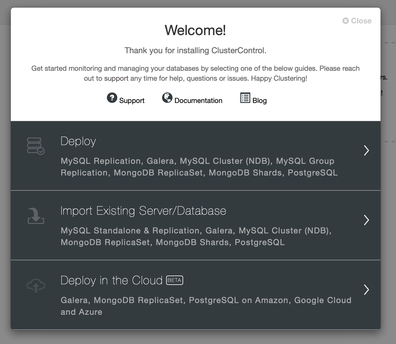
Nextcloud is an open source file sync and share application that offers free, secure, and easily accessible cloud file storage, as well as a number of tools that extend its feature set. It's very similar to the popular Dropbox, iCloud and Google Drive but unlike Dropbox, Nextcloud does not offer off-premises file storage hosting. 

In this blog post, we are going to deploy a high-available setup for our private "Dropbox" infrastructure using Nextcloud, GlusterFS, Percona XtraDB Cluster (MySQL Galera Cluster), ProxySQL with ClusterControl as the automation tool to manage and monitor the database and load balancer tiers. 

Note: You can also use MariaDB Cluster, which uses the same underlying replication library as in Percona XtraDB Cluster. From a load balancer perspective, ProxySQL behaves similarly to MaxScale in that it can understand the SQL traffic and has fine-grained control on how traffic is routed. 

Database Architecture for Nexcloud

In this blog post, we used a total of 6 nodes.

• 2 x proxy servers 
• 3 x database + application servers
• 1 x controller server (ClusterControl)

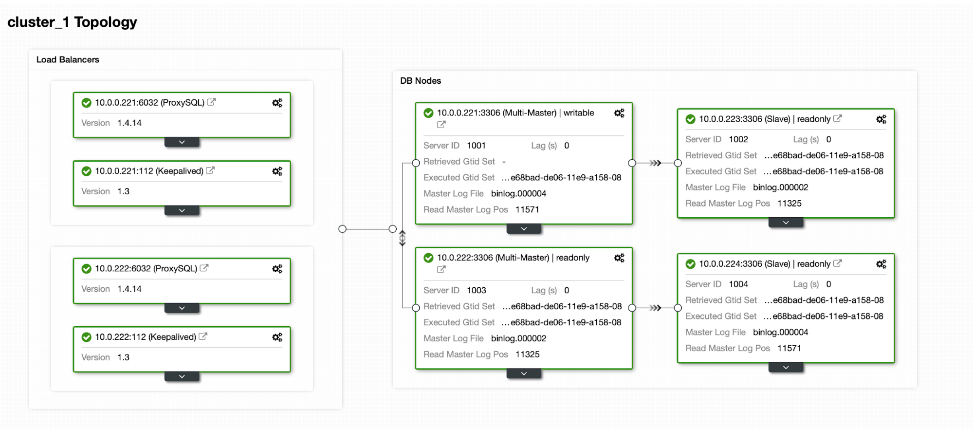
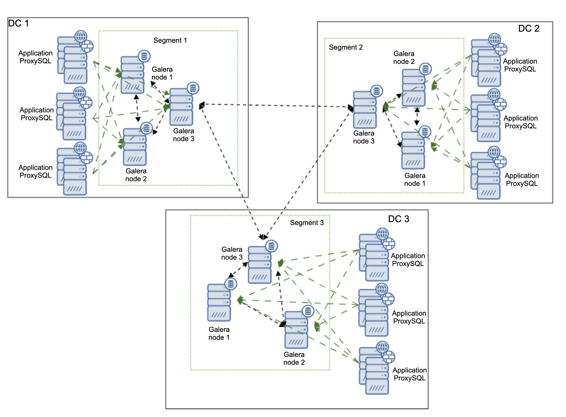
The following diagram illustrates our final setup:

For Percona XtraDB Cluster, a minimum of 3 nodes is required for a solid multi-master replication. Nextcloud applications are co-located within the database servers, thus GlusterFS has to be configured on those hosts as well. 

Load balancer tier consists of 2 nodes for redundancy purposes. We will use ClusterControl to deploy the database tier and the load balancer tiers. All servers are running on CentOS 7 with the following /etc/hosts definition on every node:

192.168.0.21 nextcloud1 db1

192.168.0.22 nextcloud2 db2

192.168.0.23 nextcloud3 db3

192.168.0.10 vip db

192.168.0.11 proxy1 lb1 proxysql1

192.168.0.12 proxy2 lb2 proxysql2

Note that GlusterFS and MySQL are highly intensive processes. If you are following this setup (GlusterFS and MySQL resides in a single server), ensure you have decent hardware specs for the servers.

Nextcloud Database Deployment

We will start with database deployment for our three-node Percona XtraDB Cluster using ClusterControl. Install ClusterControl and then setup passwordless SSH to all nodes that are going to be managed by ClusterControl (3 PXC + 2 proxies). On ClusterControl node, do:

$ whoami

root

$ ssh-copy-id 192.168.0.11

$ ssh-copy-id 192.168.0.12

$ ssh-copy-id 192.168.0.21

$ ssh-copy-id 192.168.0.22

$ ssh-copy-id 192.168.0.23

**Enter the root password for the respective host when prompted.

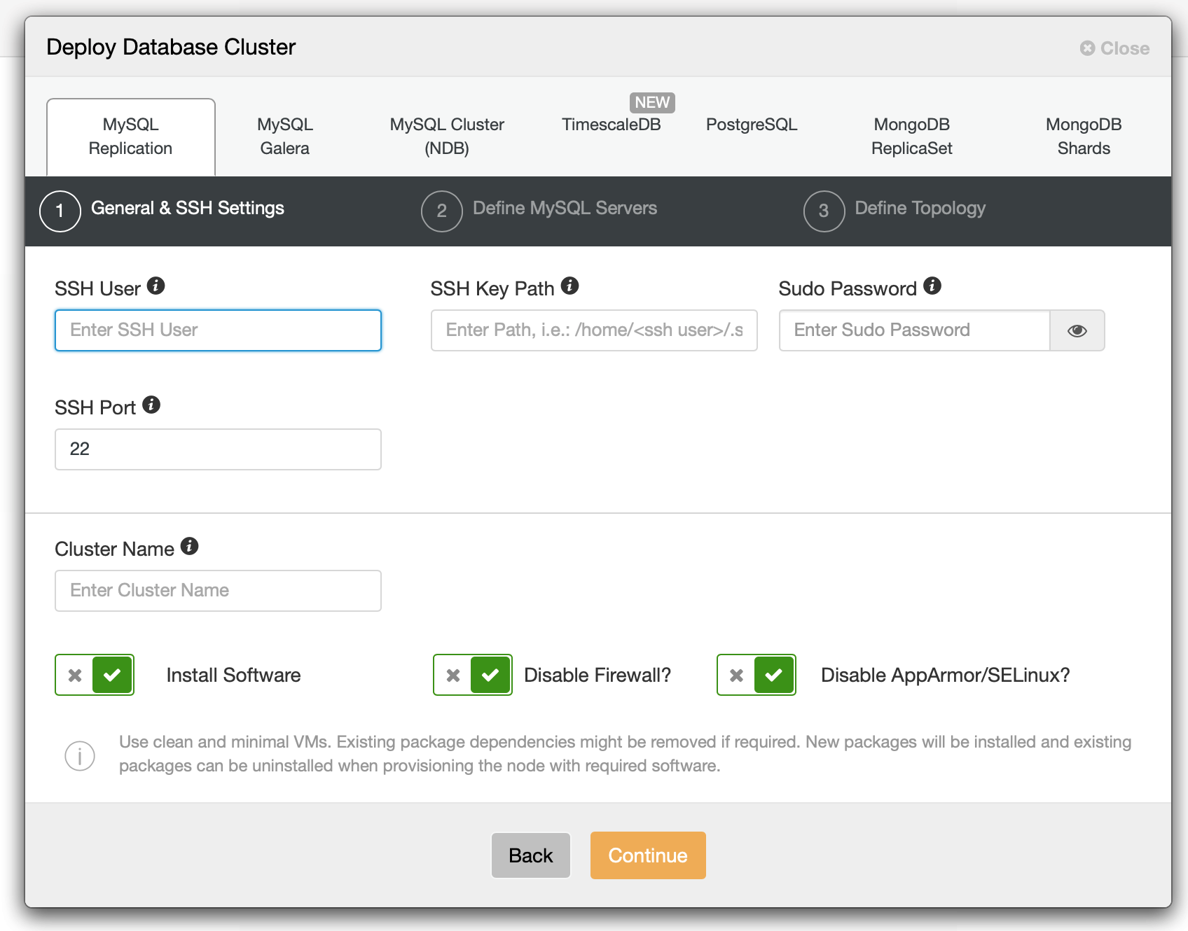
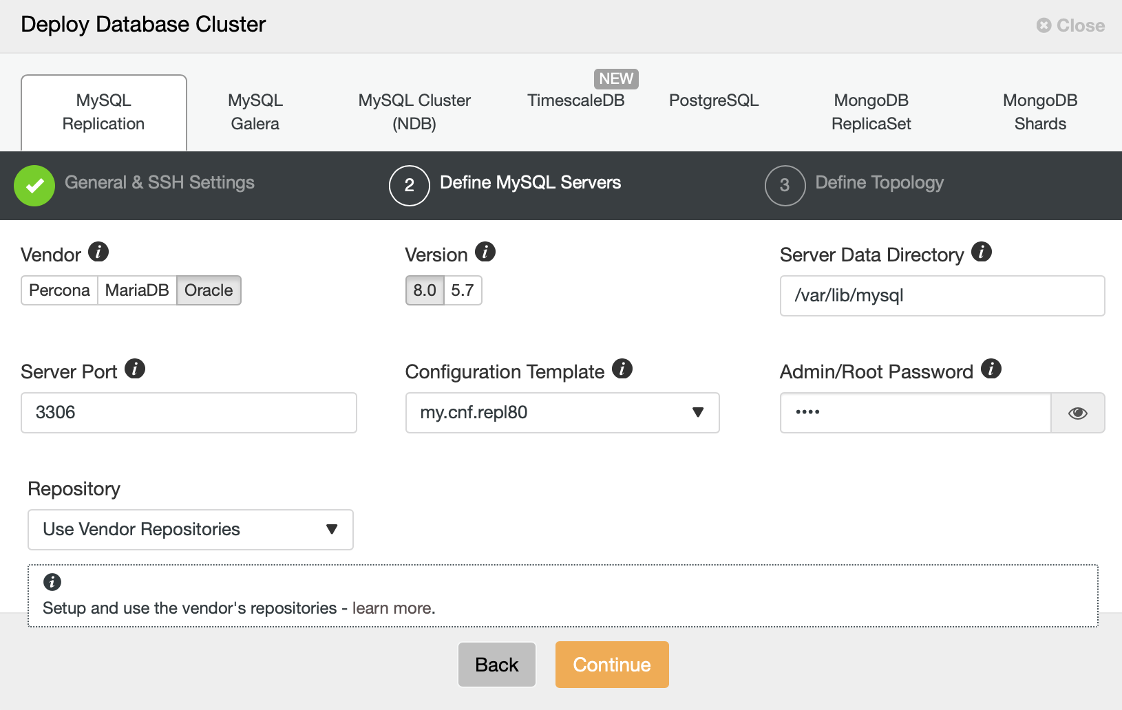
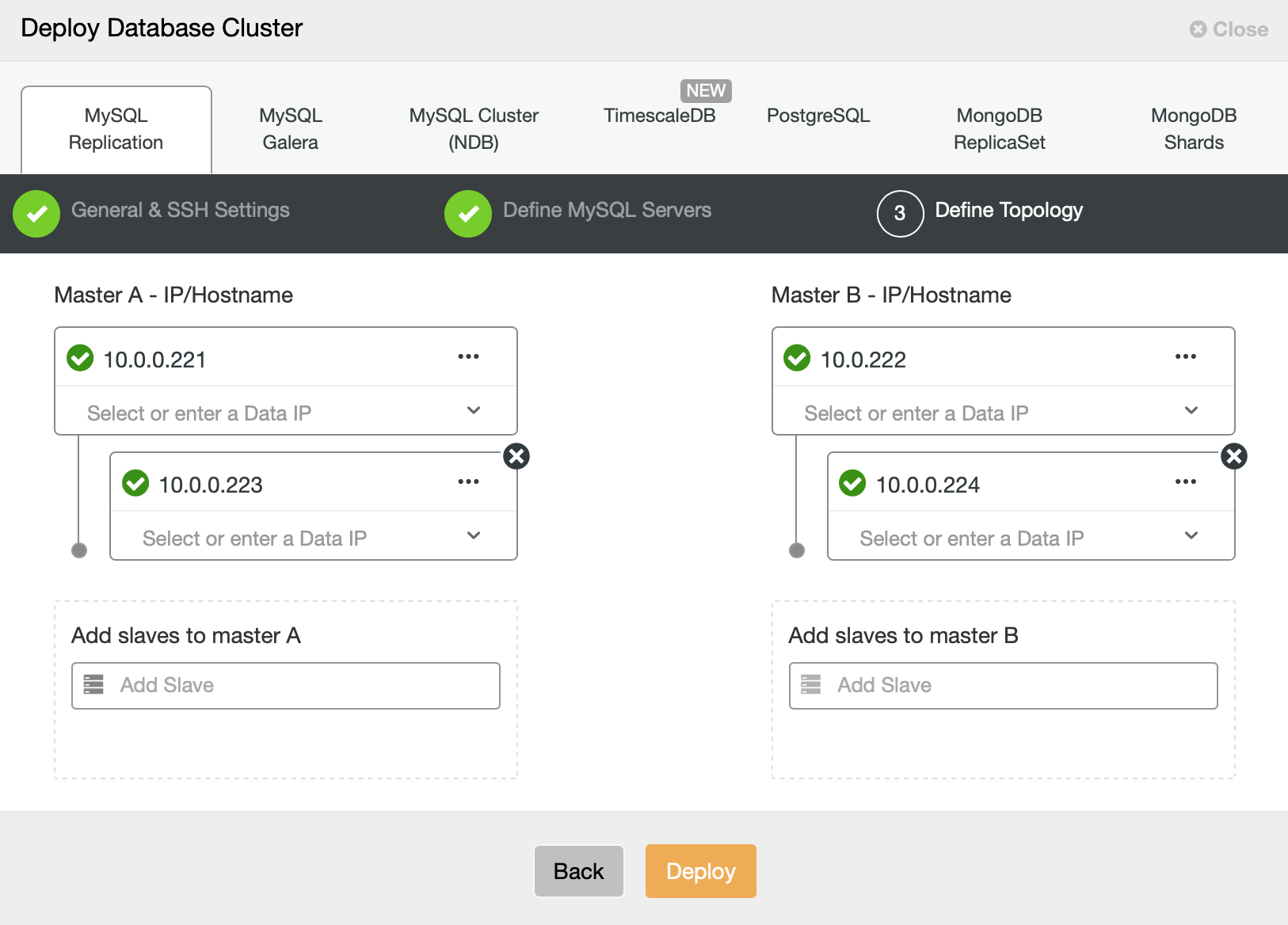
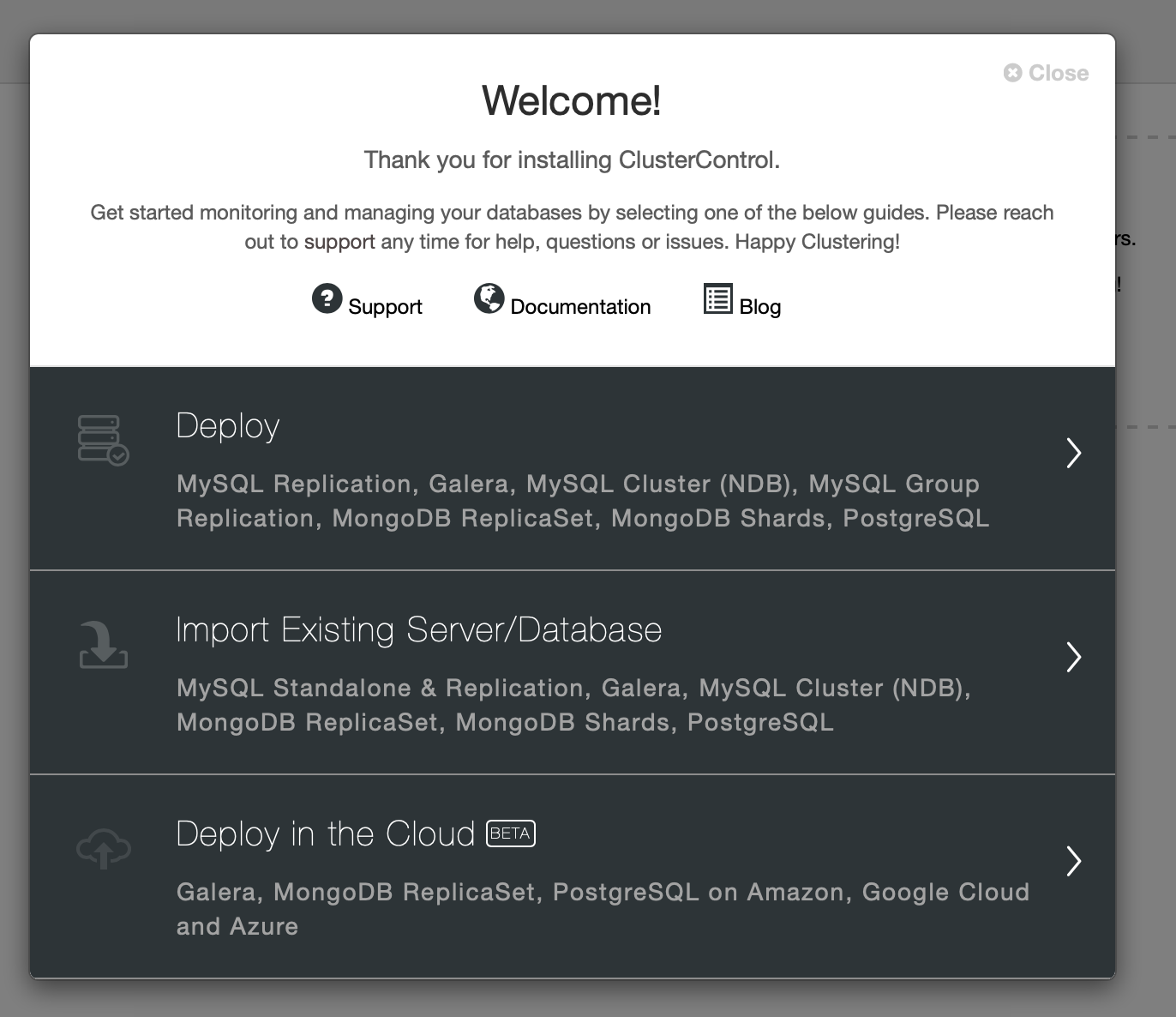
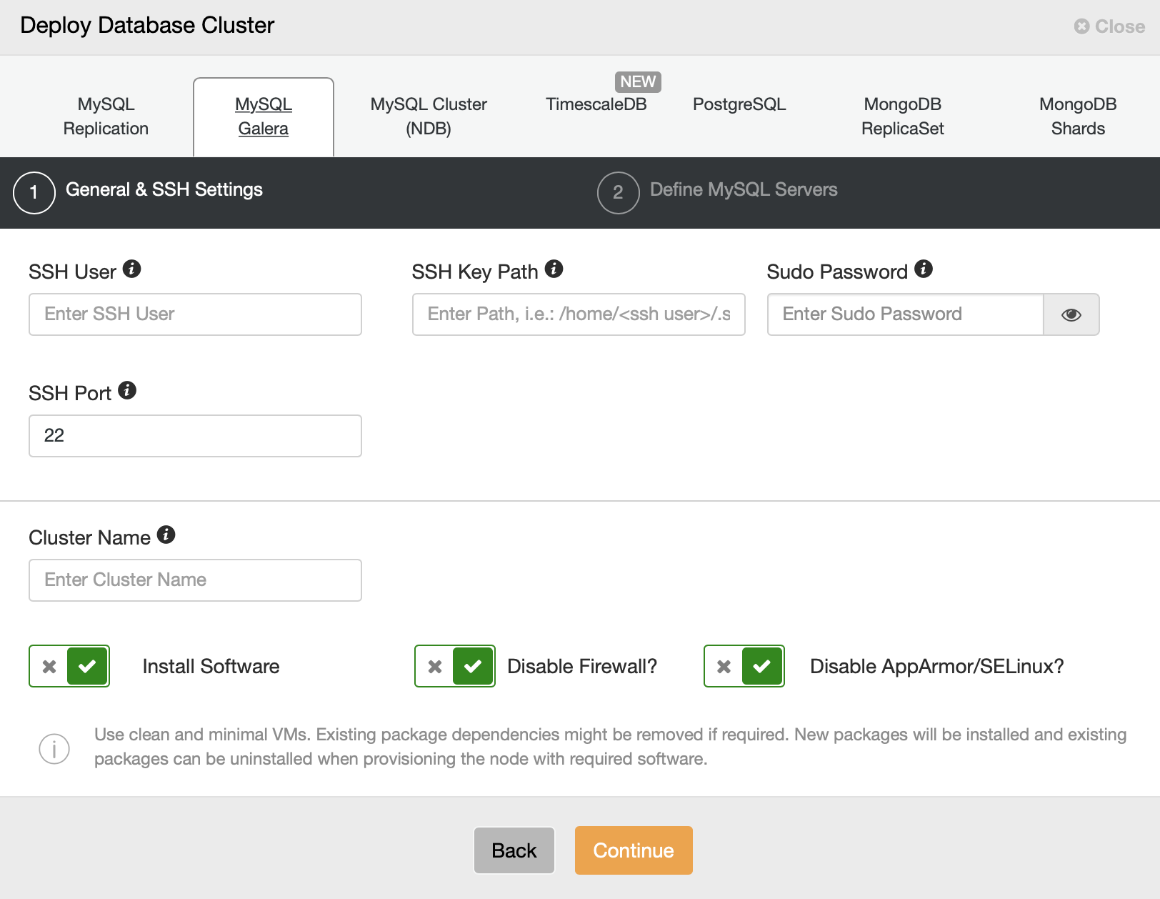
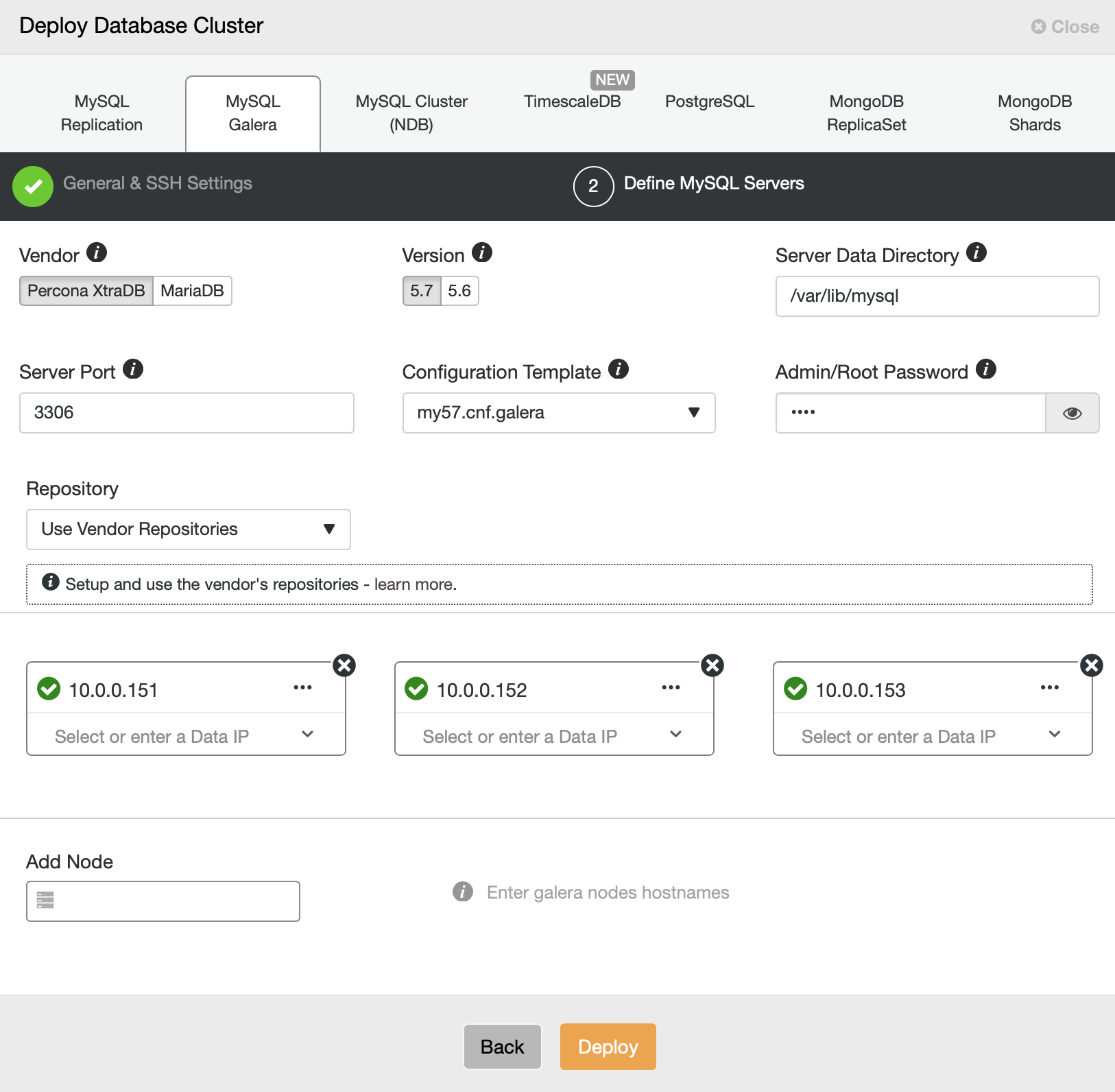
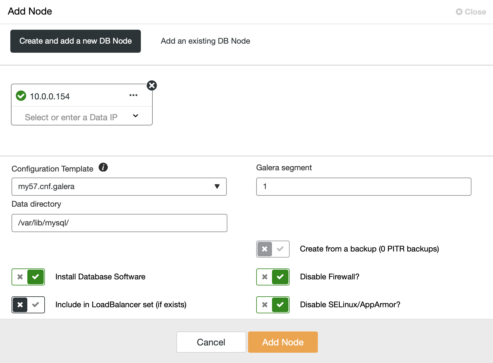
Open a web browser and go to https://{ClusterControl-IP-address}/clustercontrol and create a super user. Then go to Deploy -> MySQL Galera. Follow the deployment wizard accordingly. At the second stage 'Define MySQL Servers', pick Percona XtraDB 5.7 and specify the IP address for every database node. Make sure you get a green tick after entering the database node details, as shown below:

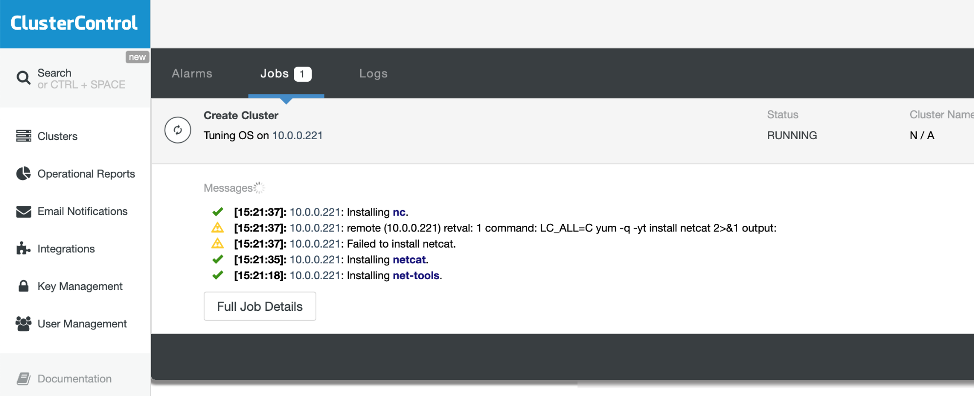
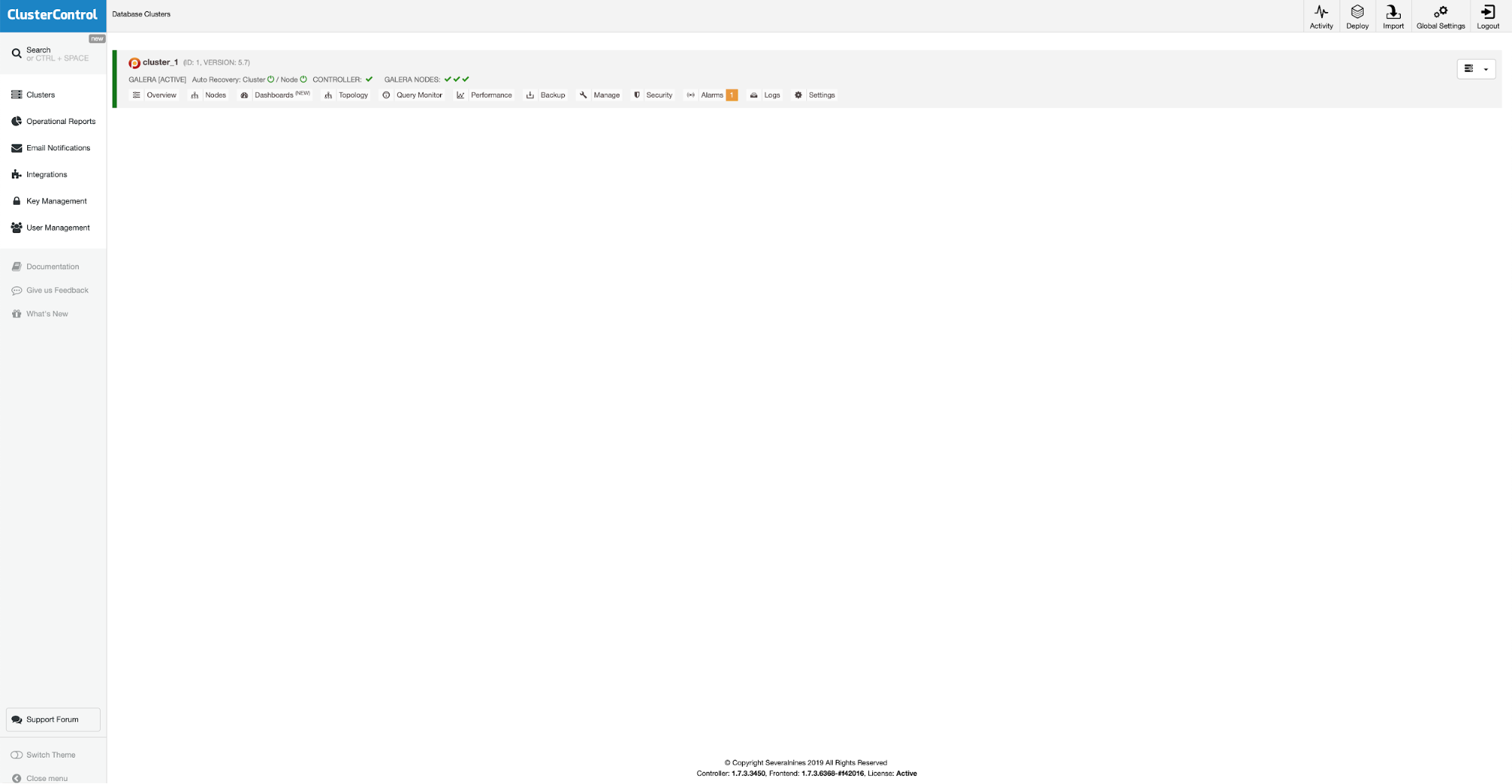
Click "Deploy" to start the deployment. The database cluster will be ready in 15~20 minutes. You can follow the deployment progress at Activity -> Jobs -> Create Cluster -> Full Job Details. The cluster will be listed under Database Cluster dashboard once deployed.

We can now proceed to database load balancer deployment.

Nextcloud Database Load Balancer Deployment

Nextcloud is recommended to run on a single-writer setup, where writes will be processed by one master at a time, and the reads can be distributed to other nodes. We can use ProxySQL 2.0 to achieve this configuration since it can route the write queries to a single master. 

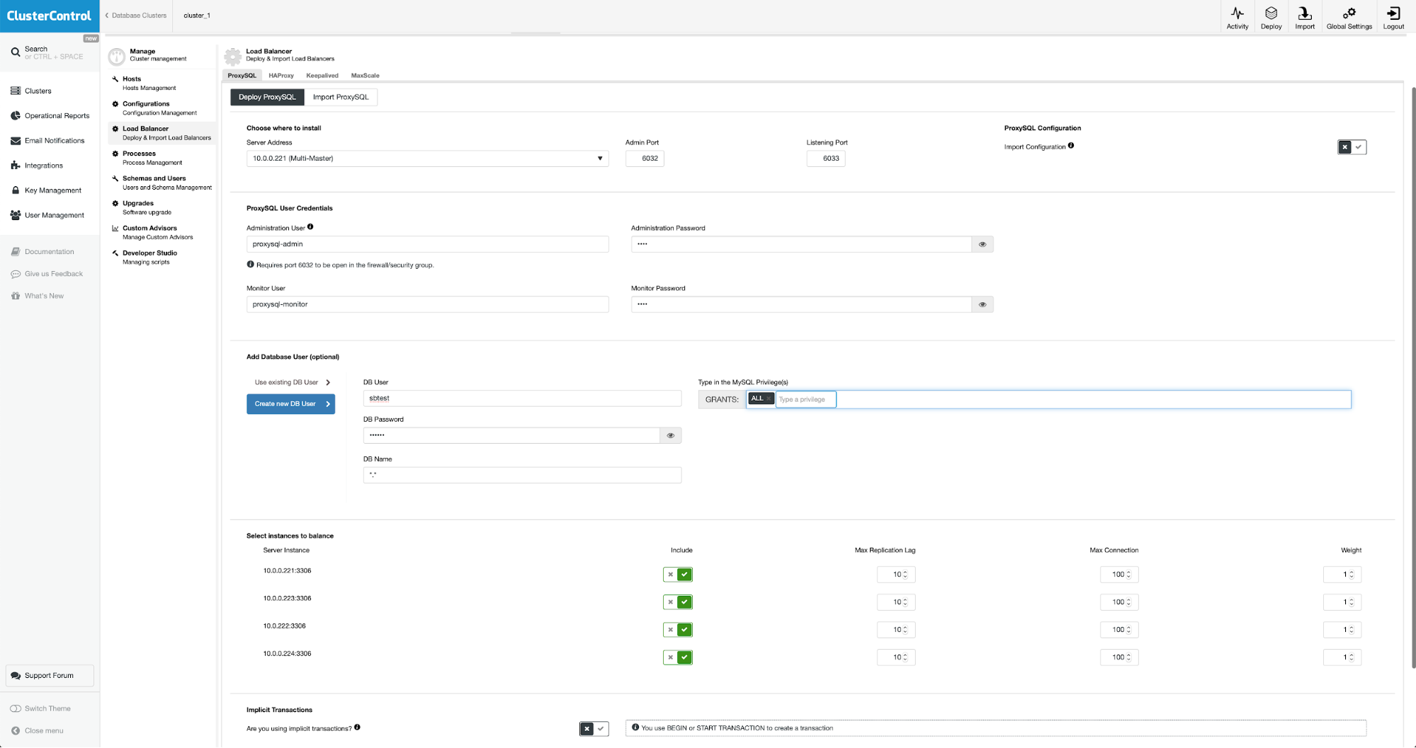
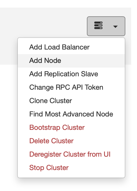
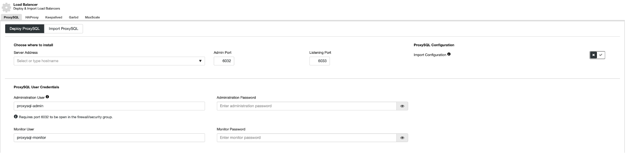
To deploy a ProxySQL, click on Cluster Actions > Add Load Balancer > ProxySQL > Deploy ProxySQL. Enter the required information as highlighted by the red arrows:

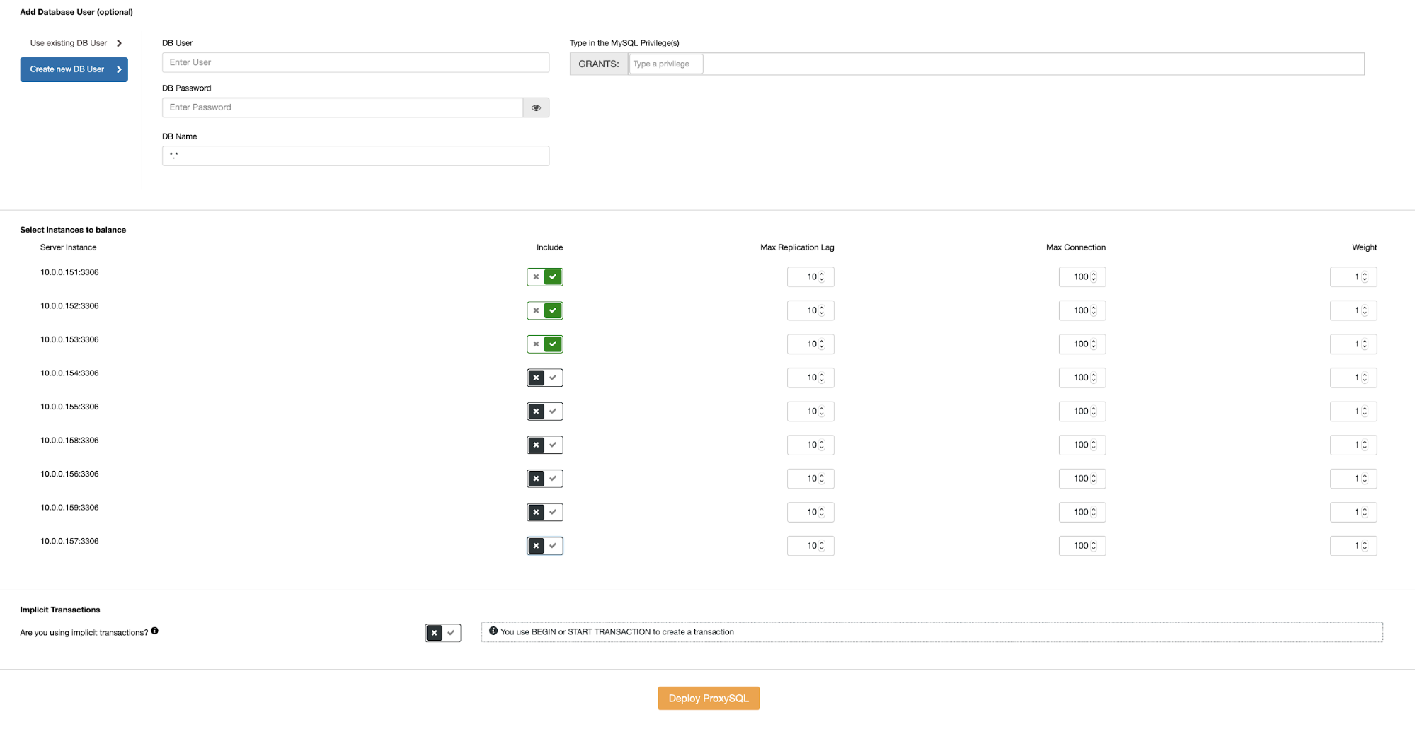
Fill in all necessary details as highlighted by the arrows above. The server address is the lb1 server, 192.168.0.11. Further down, we specify the ProxySQL admin and monitoring users' password. Then include all MySQL servers into the load balancing set and then choose "No" in the Implicit Transactions section. Click "Deploy ProxySQL" to start the deployment.

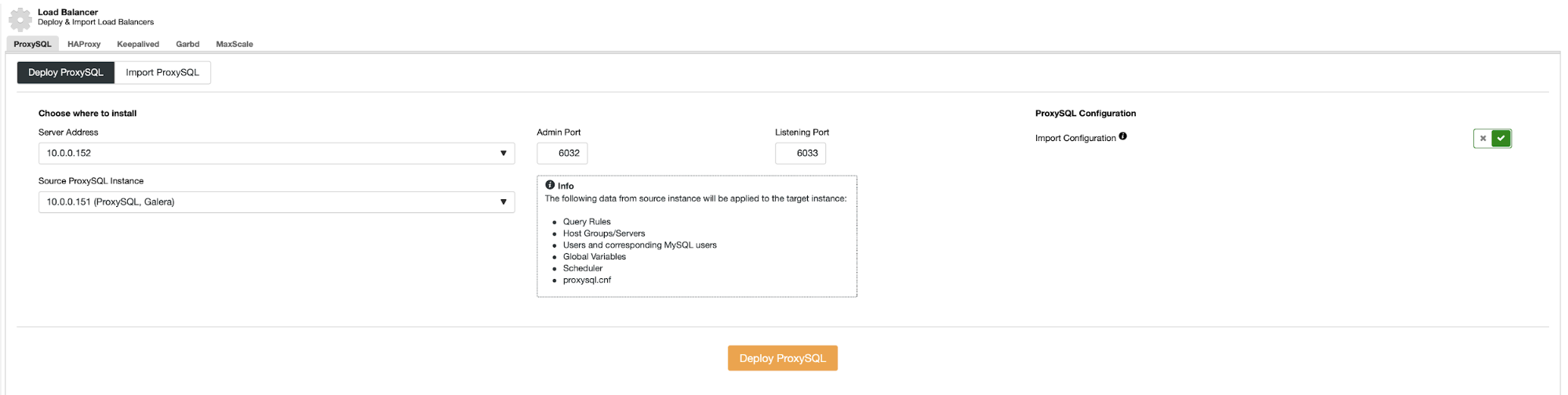
Repeat the same steps as above for the secondary load balancer, lb2 (but change the "Server Address" to lb2's IP address). Otherwise, we would have no redundancy in this layer.

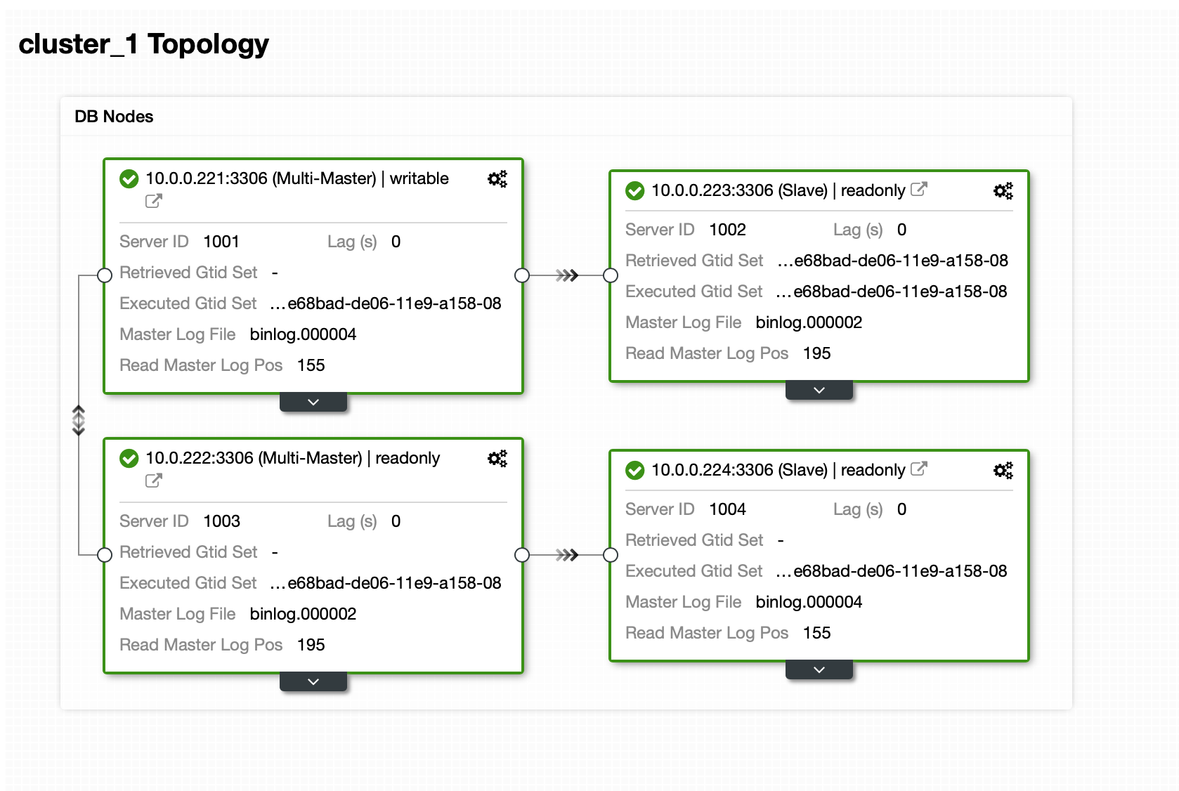
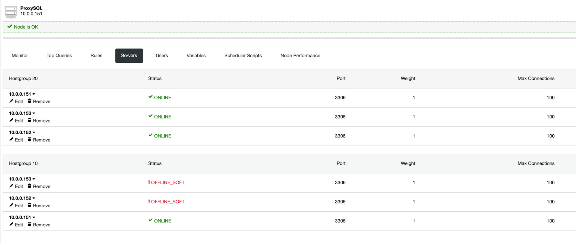
Our ProxySQL nodes are now installed and configured with two host groups for Galera Cluster. One for the single-master group (hostgroup 10), where all connections will be forwarded to one Galera node (this is useful to prevent multi-master deadlocks) and the multi-master group (hostgroup 20) for all read-only workloads which will be balanced to all backend MySQL servers.

Next, we need to deploy a virtual IP address to provide a single endpoint for our ProxySQL nodes so your application will not need to define two different ProxySQL hosts. This will also provide automatic failover capabilities because virtual IP address will be taken over by the backup ProxySQL node in case something goes wrong to the primary ProxySQL node.

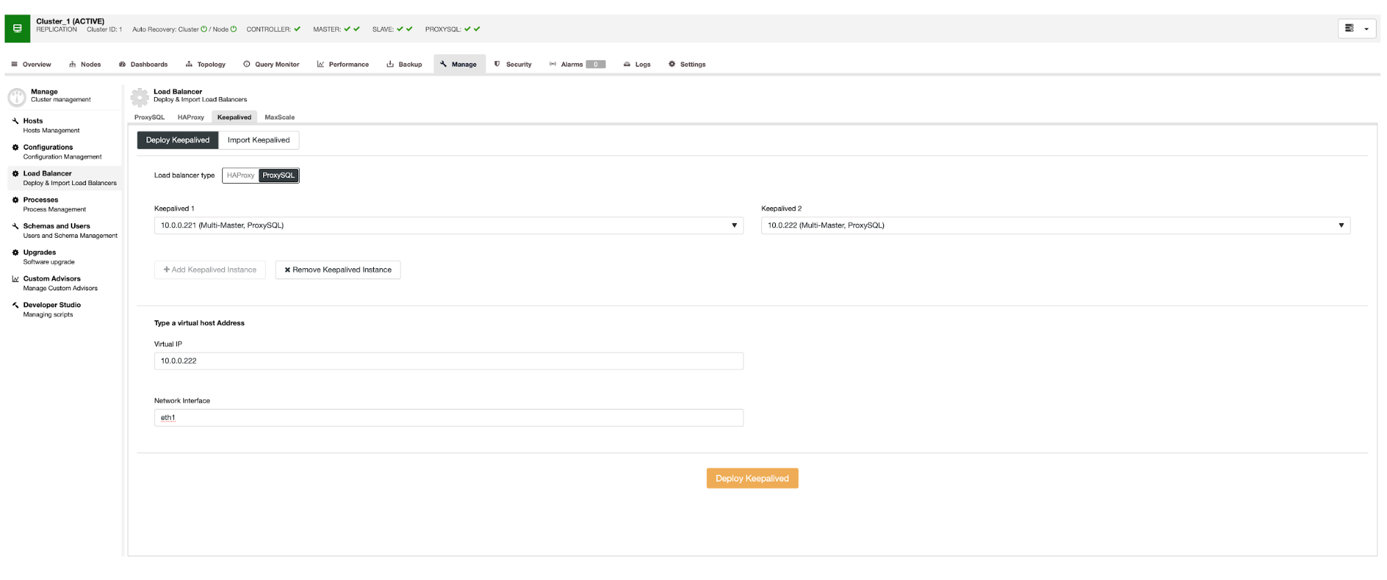
Go to ClusterControl -> Manage -> Load Balancers -> Keepalived -> Deploy Keepalived. Pick "ProxySQL" as the load balancer type and choose two distinct ProxySQL servers from the dropdown. Then specify the virtual IP address as well as the network interface that it will listen to, as shown in the following example:

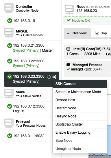
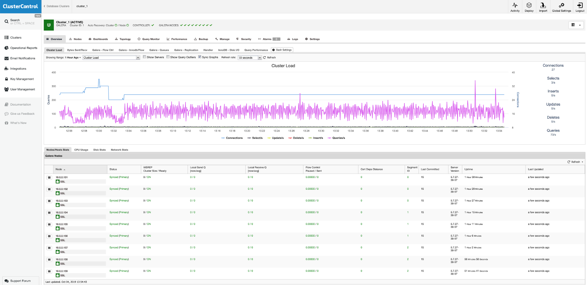
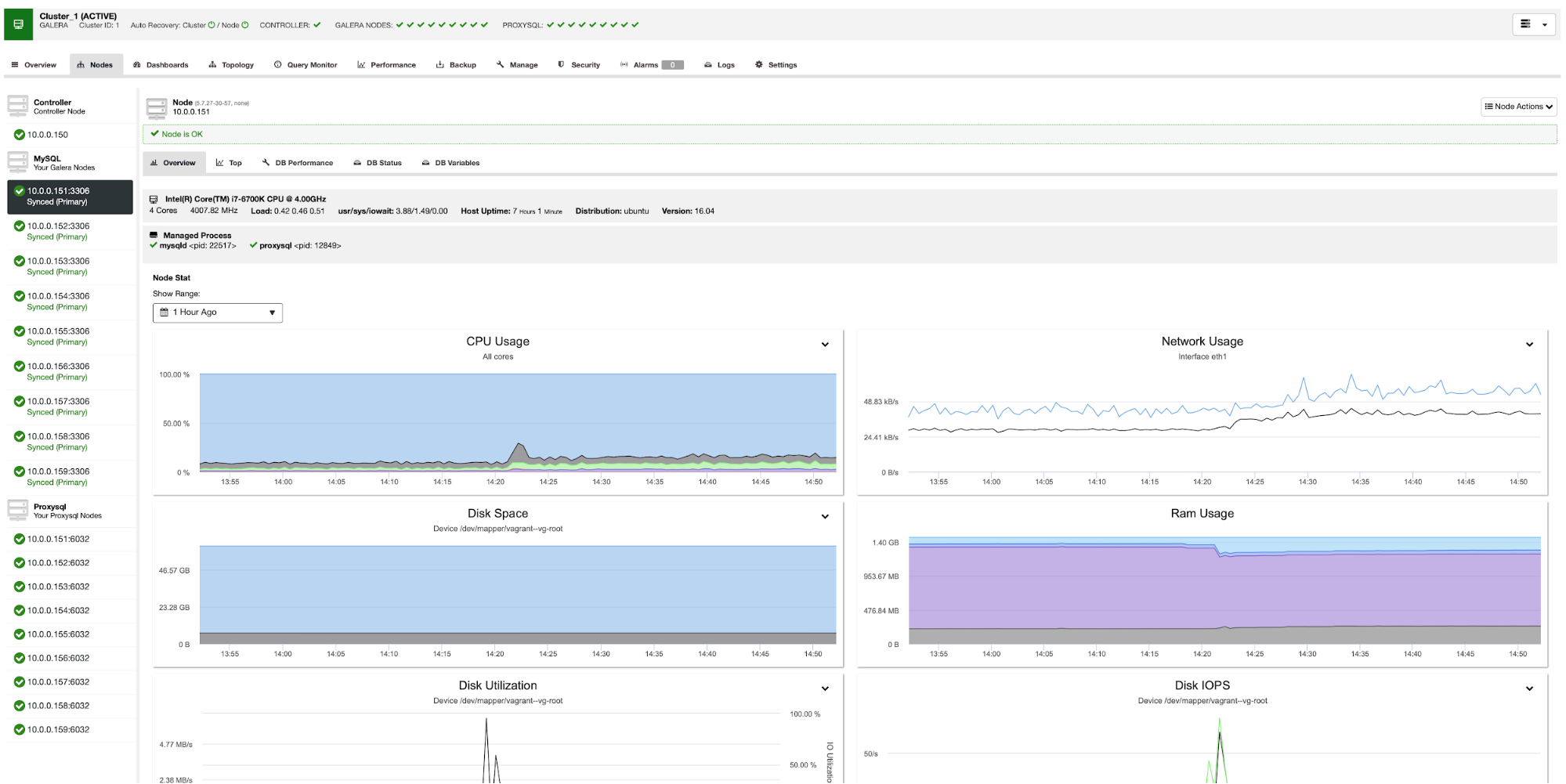
Once the deployment completes, you should see the following details on the cluster's summary bar:

Finally, create a new database for our application by going to ClusterControl -> Manage -> Schemas and Users -> Create Database and specify "nextcloud". ClusterControl will create this database on every Galera node. Our load balancer tier is now complete.

GlusterFS Deployment for Nextcloud

The following steps should be performed on nextcloud1, nextcloud2, nextcloud3 unless otherwise specified.

Step One

It's recommended to have a separate this for GlusterFS storage, so we are going to add additional disk under /dev/sdb and create a new partition:

$ fdisk /dev/sdb

Follow the fdisk partition creation wizard by pressing the following key:

n > p > Enter > Enter > Enter > w

Step Two

Verify if /dev/sdb1 has been created:

$ fdisk -l /dev/sdb1

Disk /dev/sdb1: 8588 MB, 8588886016 bytes, 16775168 sectors

Units = sectors of 1 * 512 = 512 bytes

Sector size (logical/physical): 512 bytes / 512 bytes

I/O size (minimum/optimal): 512 bytes / 512 bytes

Step Three

Format the partition with XFS:

$ mkfs.xfs /dev/sdb1

Step Four

Mount the partition as /storage/brick:

$ mkdir /glusterfs

$ mount /dev/sdb1 /glusterfs

Verify that all nodes have the following layout:

$ lsblk

NAME   MAJ:MIN RM SIZE RO TYPE MOUNTPOINT

sda      8:0 0 40G  0 disk

└─sda1   8:1 0 40G  0 part /

sdb      8:16 0   8G 0 disk

└─sdb1   8:17 0   8G 0 part /glusterfs

Step Five

Create a subdirectory called brick under /glusterfs:

$ mkdir /glusterfs/brick

Step Six

For application redundancy, we can use GlusterFS for file replication between the hosts. Firstly, install GlusterFS repository for CentOS:

$ yum install centos-release-gluster -y

$ yum install epel-release -y

Step Seven

Install GlusterFS server

$ yum install glusterfs-server -y

Step Eight

Enable and start gluster daemon:

$ systemctl enable glusterd

$ systemctl start glusterd

Step Nine

On nextcloud1, probe the other nodes:

(nextcloud1)$ gluster peer probe 192.168.0.22

(nextcloud1)$ gluster peer probe 192.168.0.23

You can verify the peer status with the following command:

(nextcloud1)$ gluster peer status

Number of Peers: 2



Hostname: 192.168.0.22

Uuid: f9d2928a-6b64-455a-9e0e-654a1ebbc320

State: Peer in Cluster (Connected)



Hostname: 192.168.0.23

Uuid: 100b7778-459d-4c48-9ea8-bb8fe33d9493

State: Peer in Cluster (Connected)

Step Ten

On nextcloud1, create a replicated volume on probed nodes:

(nextcloud1)$ gluster volume create rep-volume replica 3 192.168.0.21:/glusterfs/brick 192.168.0.22:/glusterfs/brick 192.168.0.23:/glusterfs/brick

volume create: rep-volume: success: please start the volume to access data

Step Eleven

Start the replicated volume on nextcloud1:

(nextcloud1)$ gluster volume start rep-volume

volume start: rep-volume: success

Verify the replicated volume and processes are online:

$ gluster volume status

Status of volume: rep-volume

Gluster process                             TCP Port RDMA Port Online Pid

------------------------------------------------------------------------------

Brick 192.168.0.21:/glusterfs/brick         49152 0 Y 32570

Brick 192.168.0.22:/glusterfs/brick         49152 0 Y 27175

Brick 192.168.0.23:/glusterfs/brick         49152 0 Y 25799

Self-heal Daemon on localhost               N/A N/A Y 32591

Self-heal Daemon on 192.168.0.22            N/A N/A Y 27196

Self-heal Daemon on 192.168.0.23            N/A N/A Y 25820



Task Status of Volume rep-volume

------------------------------------------------------------------------------

There are no active volume tasks

Step Twelve

Mount the replicated volume on /var/www/html. Create the directory:

$ mkdir -p /var/www/html

Step Thirteen

13) Add following line into /etc/fstab to allow auto-mount:

/dev/sdb1 /glusterfs xfs defaults,defaults 0 0

localhost:/rep-volume /var/www/html   glusterfs defaults,_netdev 0 0

Step Fourteen

Mount the GlusterFS to /var/www/html:

$ mount -a

And verify with:

$ mount | grep gluster

/dev/sdb1 on /glusterfs type xfs (rw,relatime,seclabel,attr2,inode64,noquota)

localhost:/rep-volume on /var/www/html type fuse.glusterfs (rw,relatime,user_id=0,group_id=0,default_permissions,allow_other,max_read=131072)

The replicated volume is now ready and mounted in every node. We can now proceed to deploy the application.

Nextcloud Application Deployment

The following steps should be performed on nextcloud1, nextcloud2 and nextcloud3 unless otherwise specified.

Nextcloud requires PHP 7.2 and later and for CentOS distribution, we have to enable a number of repositories like EPEL and Remi to simplify the installation process.

Step One

If SELinux is enabled, disable it first:

$ setenforce 0

$ sed -i 's/^SELINUX=.*/SELINUX=permissive/g' /etc/selinux/config

You can also run Nextcloud with SELinux enabled by following this guide.

Step Two

Install Nextcloud requirements and enable Remi repository for PHP 7.2:

$ yum install -y epel-release yum-utils unzip curl wget bash-completion policycoreutils-python mlocate bzip2

$ yum install -y http://rpms.remirepo.net/enterprise/remi-release-7.rpm

$ yum-config-manager --enable remi-php72

Step Three

Install Nextcloud dependencies, mostly Apache and PHP 7.2 related packages:

$ yum install -y httpd php72-php php72-php-gd php72-php-intl php72-php-mbstring php72-php-mysqlnd php72-php-opcache php72-php-pecl-redis php72-php-pecl-apcu php72-php-pecl-imagick php72-php-xml php72-php-pecl-zip

Step Four

Enable Apache and start it up:

$ systemctl enable httpd.service

$ systemctl start httpd.service

Step Five

Make a symbolic link for PHP to use PHP 7.2 binary:

$ ln -sf /bin/php72 /bin/php

Step Six

On nextcloud1, download Nextcloud Server from here and extract it:

$ wget https://download.nextcloud.com/server/releases/nextcloud-17.0.0.zip

$ unzip nextcloud*

Step Seven

On nextcloud1, copy the directory into /var/www/html and assign correct ownership:

$ cp -Rf nextcloud /var/www/html

$ chown -Rf apache:apache /var/www/html

**Note the copying process into /var/www/html is going to take some time due to GlusterFS volume replication.

Step Eight

Before we proceed to open the installation wizard, we have to disable pxc_strict_mode variable to other than "ENFORCING" (the default value). This is due to the fact that Nextcloud database import will have a number of tables without primary key defined which is not recommended to run on Galera Cluster. This is explained further details under Tuning section further down.

To change the configuration with ClusterControl, simply go to Manage -> Configurations -> Change/Set Parameters:

Choose all database instances from the list, and enter:

• Group: MYSQLD
• Parameter: pxc_strict_mode
• New Value: PERMISSIVE

ClusterControl will perform the necessary changes on every database node automatically. If the value can be changed during runtime, it will be effective immediately. ClusterControl also configure the value inside MySQL configuration file for persistency. You should see the following result:

Step Nine

Now we are ready to configure our Nextcloud installation. Open the browser and go to nextcloud1's HTTP server at http://192.168.0.21/nextcloud/ and you will be presented with the following configuration wizard:

Configure the "Storage & database" section with the following value:

• Data folder: /var/www/html/nextcloud/data
• Configure the database: MySQL/MariaDB
• Username: nextcloud
• Password: (the password for user nextcloud)
• Database: nextcloud
• Host: 192.168.0.10:6603 (The virtual IP address with ProxySQL port)

Click "Finish Setup" to start the configuration process. Wait until it finishes and you will be redirected to Nextcloud dashboard for user "admin". The installation is now complete. Next section provides some tuning tips to run efficiently with Galera Cluster.

Nextcloud Database Tuning

Primary Key

Having a primary key on every table is vital for Galera Cluster write-set replication. For a relatively big table without primary key, large update or delete transaction would completely block your cluster for a very long time. To avoid any quirks and edge cases, simply make sure that all tables are using InnoDB storage engine with an explicit primary key (unique key does not count).

The default installation of Nextcloud will create a bunch of tables under the specified database and some of them do not comply with this rule. To check if the tables are compatible with Galera, we can run the following statement:

mysql> SELECT DISTINCT CONCAT(t.table_schema,'.',t.table_name) as tbl, t.engine, IF(ISNULL(c.constraint_name),'NOPK','') AS nopk, IF(s.index_type = 'FULLTEXT','FULLTEXT','') as ftidx, IF(s.index_type = 'SPATIAL','SPATIAL','') as gisidx FROM information_schema.tables AS t LEFT JOIN information_schema.key_column_usage AS c ON (t.table_schema = c.constraint_schema AND t.table_name = c.table_name AND c.constraint_name = 'PRIMARY') LEFT JOIN information_schema.statistics AS s ON (t.table_schema = s.table_schema AND t.table_name = s.table_name AND s.index_type IN ('FULLTEXT','SPATIAL'))   WHERE t.table_schema NOT IN ('information_schema','performance_schema','mysql') AND t.table_type = 'BASE TABLE' AND (t.engine <> 'InnoDB' OR c.constraint_name IS NULL OR s.index_type IN ('FULLTEXT','SPATIAL')) ORDER BY t.table_schema,t.table_name;

+---------------------------------------+--------+------+-------+--------+

| tbl                                   | engine | nopk | ftidx | gisidx |

+---------------------------------------+--------+------+-------+--------+

| nextcloud.oc_collres_accesscache      | InnoDB | NOPK | | |

| nextcloud.oc_collres_resources        | InnoDB | NOPK | | |

| nextcloud.oc_comments_read_markers    | InnoDB | NOPK | | |

| nextcloud.oc_federated_reshares       | InnoDB | NOPK | | |

| nextcloud.oc_filecache_extended       | InnoDB | NOPK | | |

| nextcloud.oc_notifications_pushtokens | InnoDB | NOPK |       | |

| nextcloud.oc_systemtag_object_mapping | InnoDB | NOPK |       | |

+---------------------------------------+--------+------+-------+--------+

The above output shows there are 7 tables that do not have a primary key defined. To fix the above, simply add a primary key with auto-increment column. Run the following commands on one of the database servers, for example nexcloud1:

(nextcloud1)$ mysql -uroot -p

mysql> ALTER TABLE nextcloud.oc_collres_accesscache ADD COLUMN `id` INT PRIMARY KEY AUTO_INCREMENT;

mysql> ALTER TABLE nextcloud.oc_collres_resources ADD COLUMN `id` INT PRIMARY KEY AUTO_INCREMENT;

mysql> ALTER TABLE nextcloud.oc_comments_read_markers ADD COLUMN `id` INT PRIMARY KEY AUTO_INCREMENT;

mysql> ALTER TABLE nextcloud.oc_federated_reshares ADD COLUMN `id` INT PRIMARY KEY AUTO_INCREMENT;

mysql> ALTER TABLE nextcloud.oc_filecache_extended ADD COLUMN `id` INT PRIMARY KEY AUTO_INCREMENT;

mysql> ALTER TABLE nextcloud.oc_notifications_pushtokens ADD COLUMN `id` INT PRIMARY KEY AUTO_INCREMENT;

mysql> ALTER TABLE nextcloud.oc_systemtag_object_mapping ADD COLUMN `id` INT PRIMARY KEY AUTO_INCREMENT;

Once the above modifications have been applied, we can reconfigure back the pxc_strict_mode to the recommended value, "ENFORCING". Repeat step #8 under "Application Deployment" section with the corresponding value.

READ-COMMITTED Isolation Level

The recommended transaction isolation level as advised by Nextcloud is to use READ-COMMITTED, while Galera Cluster is default to stricter REPEATABLE-READ isolation level. Using READ-COMMITTED can avoid data loss under high load scenarios (e.g. by using the sync client with many clients/users and many parallel operations).

To modify the transaction level, go to ClusterControl -> Manage -> Configurations -> Change/Set Parameter and specify the following:

Click "Proceed" and ClusterControl will apply the configuration changes immediately. No database restart is required.

Multi-Instance Nextcloud

Since we performed the installation on nextcloud1 when accessing the URL, this IP address is automatically added into 'trusted_domains' variable inside Nextcloud. When you tried to access other servers, for example the secondary server, http://192.168.0.22/nextcloud, you would see an error that this is host is not authorized and must be added into the trusted_domain variable.

Therefore, add all the hosts IP address under "trusted_domain" array inside /var/www/html/nextcloud/config/config.php, as example below:

'trusted_domains' =>

  array (

    0 => '192.168.0.21',

    1 => '192.168.0.22',

    2 => '192.168.0.23'

  ),

The above configuration allows users to access all three application servers via the following URLs:

• http://192.168.0.21/nextcloud (nextcloud1)
• http://192.168.0.22/nextcloud (nextcloud2)
• http://192.168.0.23/nextcloud (nextcloud3)

Note: You can add a load balancer tier on top of these three Nextcloud instances to achieve high availability for the application tier by using HTTP reverse proxies available in the market like HAProxy or nginx. That is out of the scope of this blog post.

Using Redis for File Locking

Nextcloud’s Transactional File Locking mechanism locks files to avoid file corruption during normal operation. It's recommended to install Redis to take care of transactional file locking (this is enabled by default) which will offload the database cluster from handling this heavy job.

To install Redis, simply:

$ yum install -y redis

$ systemctl enable redis.service

$ systemctl start redis.service

Append the following lines inside /var/www/html/nextcloud/config/config.php:

'filelocking.enabled' => true,

  'memcache.locking' => '\OC\Memcache\Redis',

  'redis' => array(

     'host' => '192.168.0.21',

     'port' => 6379,

     'timeout' => 0.0,

   ),

For more details, check out this documentation, Transactional File Locking.

Conclusion

Nextcloud can be configured to be a scalable and highly available file-hosting service to cater for your private file sharing demands. In this blog, we showed how you can bring redundancy in the Nextcloud, file system and database layers. 

When a project is being designed, the first thing to think about is what its purpose will be... what is the best solution, and what are the alternatives.  In software engineering, everything is done to serve data, whether it's a graphical interface or business logic, so it's no wonder the best starting point might be database planning.

The official documentation of a database can be very complicated, whatever technology it may be. Using the best concepts for a specific situation is not an easy task.

pgModeler is the program you can use to increase your productivity with PostgreSQL. It's free, works on Windows, Mac, or Linux and provides a way to work with DDL commands through a rich interface built on top of SVG.

Installation

Installation is very simple, just download it from the site, and run the file. Some operating systems already have pgModeler included in their repositories, which is an alternative to downloading it.

pgModeler is an open source solution, and you can find it on GitHub, where new releases are published. 

It has a  paid version option, where you can support the project and use the latest features, for example, compatibility with the latest versions of PostgreSQL.

If you need a desktop entry, check it out in the following. This file can be named pgmodeler.desktop, and you can place it on /usr/share/applications/, but don’t forget to copy the logo presented in this blog, saving it on /etc/pgmodeler/pgmodeler_logo.png.

[Desktop Entry]
Name=pgModeler
GenericName=PostgreSQL Database Modeler
Comment=Program with nice Qt interface for visual modeling PostgreSQL on Entity Relationship Diagram
Exec=pgmodeler
Icon=/etc/pgmodeler/pgmodeler_logo.png
Terminal=false
Type=Application
Categories=Qt;Database;Development;

Graphical Interface

The curriculum of information technology courses, including colleges, contains data modeling disciplines, with UML as the standard for project design and documentation.

The graphical interface of pgModeler allows working with a kind of diagram specific for databases, the Entity Relationship Diagram (ERD), reproducing what you’ve built inside of your PostgreSQL cluster seamlessly.

Several languages are available:

• English (en_US);
• Spanish (es_ES);
• French (fr_FR);
• Dutch (nl_NL);
• Portuguese (pt_BR); and
• Chinese (zh_CN).

Printing what you’ve built is also available, and customizations are possible in the appearance, changing the font and colors of schemas, tables, relationships, etc.

Features

The features of pgModeler are simply tools to help you navigate between logical and physical models.

A logical model, is the diagram. You can use it to transform the idea of your customer, into a well documented project that other person can understand in the future, and make modifications on it.

The physical model is the script, the SQL code. PostgreSQL understands it, and so pgModeler too.

Through its reverse engineering algorithm, you can connect into your PostgreSQL cluster, and look at your existing domain model with a different perspective, or build it first, and then create the domain model executing the script, generated by what you’ve built in the diagram.

Entity Relationship Diagram

Once you understand its purpose, let’s see how a diagram looks like for a very simple project where you can visualize the relationship between the tables customer and film, named rental.

Note the lines between the tables, they are easy to see, and most importantly, understand. Primary and foreign keys are the starting points to visualize the relationships, and at their edges, the cardinality is being shown.

The constraints representing the keys can be seen, as pk, fk, and even the NOT NULL, as nn, in green at the right of each table. The schema is named store, and the picture above has been generated by the program itself.

Earlier we saw that diagrams are the logical model, which can be applied into a PostgreSQL cluster. In order to apply it, a connection must be established, for this example, I created a cluster running inside a Docker container.

Now with the database connection configured and tested, exporting is easy. Security concerns must be considered at this point, like establishing SSL with your cluster.

In the following, pgModeler creates the store schema, inside of a completely new database named blog_db, as I wanted to, not forgetting to mention the new role, with login permission.

Exporting process successfully ended! – Ok, there is a mistake, but it has been successfully ended, for sure.

postgres@716f75fdea56:~$ psql -U thiago -w -d blog_db;
psql (10.10 (Debian 10.10-1.pgdg90+1))
Type "help" for help.
blog_db=> set search_path to store;
SET
blog_db=> \dt
        List of relations
Schema |   Name | Type  | Owner
--------+----------+-------+--------
store  | customer | table | thiago
store  | film   | table | thiago
store  | rental   | table | thiago
(3 rows)
blog_db=> \du
                                  List of roles
Role name |                         Attributes | Member of
-----------+------------------------------------------------------------+-----------
postgres  | Superuser, Create role, Create DB, Replication, Bypass RLS | {}
thiago    |                                                   | {}

Conclusion

Domain models are also known as mini worlds, and rarely you’ll see the same being applied on different projects. pgModeler can help you focus on what is really important, avoiding waste of time concerning the SQL syntax.